Chapter 12 TPC Pipelines(2)
12.1 General steps
S1: Preset — Set personalized samples and tumor data with following general steps.
- “Modify datasets”: View the dataset sources for each molecular type. When there are alternative datasets for the same molecular type, users can switch a suitable one based on purpose (referring to Chapter 10).
- “Choose cancer”: Choose one cancer type for downstream association analysis.
- “Filter samples”: Upon the selection of one tumor, further refine the samples based on tissue codes or personalized filtering module.
- “Upload metadata”: Upload user-defined tumor data for joint analysis.
- “Add signature”: Design custom molecular signature for joint analysis.
S2: Get data — Select and fetch identifier values; set grouping information.
S3: Analyze & Visualize — Modify diverse parameters; perform analysis; download results.
- “Set analyzation parameters”: Select different statistical methods
- “Set visualization parameters”: Adjust plot color, title text, etc.
- “Download results”: Download three types of results, including raw data, detailed statistical results and plot results. (Note: No plot for batch-screen mode).
Notes: We will introduce various analysis scenarios of TPC using TCGA as example.
12.2 Correlation analysis
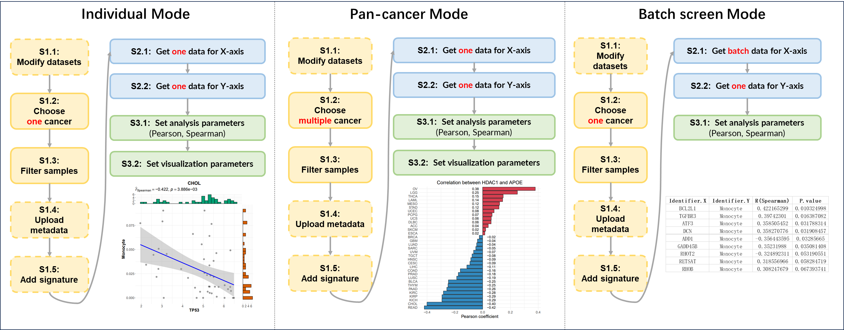
Figure 12.1: 3 modes of correlation analysis
12.2.1 Individual Mode
Perform the correlation analysis between any two identifiers of samples from one tumor.
The following is a simple example. (The steps not mentioned in above figure imply default operations.)
S1: Preset
- “S1.2 Choose cancer”: choose the CHOL (Cholangiocarcinoma) cancer type
- “S1.3 Filter samples”: choose the primary tumor samples via the quick filter.
S2: Get data
- “S2.1 Get data for X-axis”: Molecular profile→mRNA Expression→TP53
- “S2.2 Get data for Y-axis”: Infiltration→CIBERSORT→ Monocyte
S3: Analyze & Visualize
- “S3.1 Set analysis parameters”: Spearman
- “S3.2 Set visualization parameters”: Adjust the main title name.
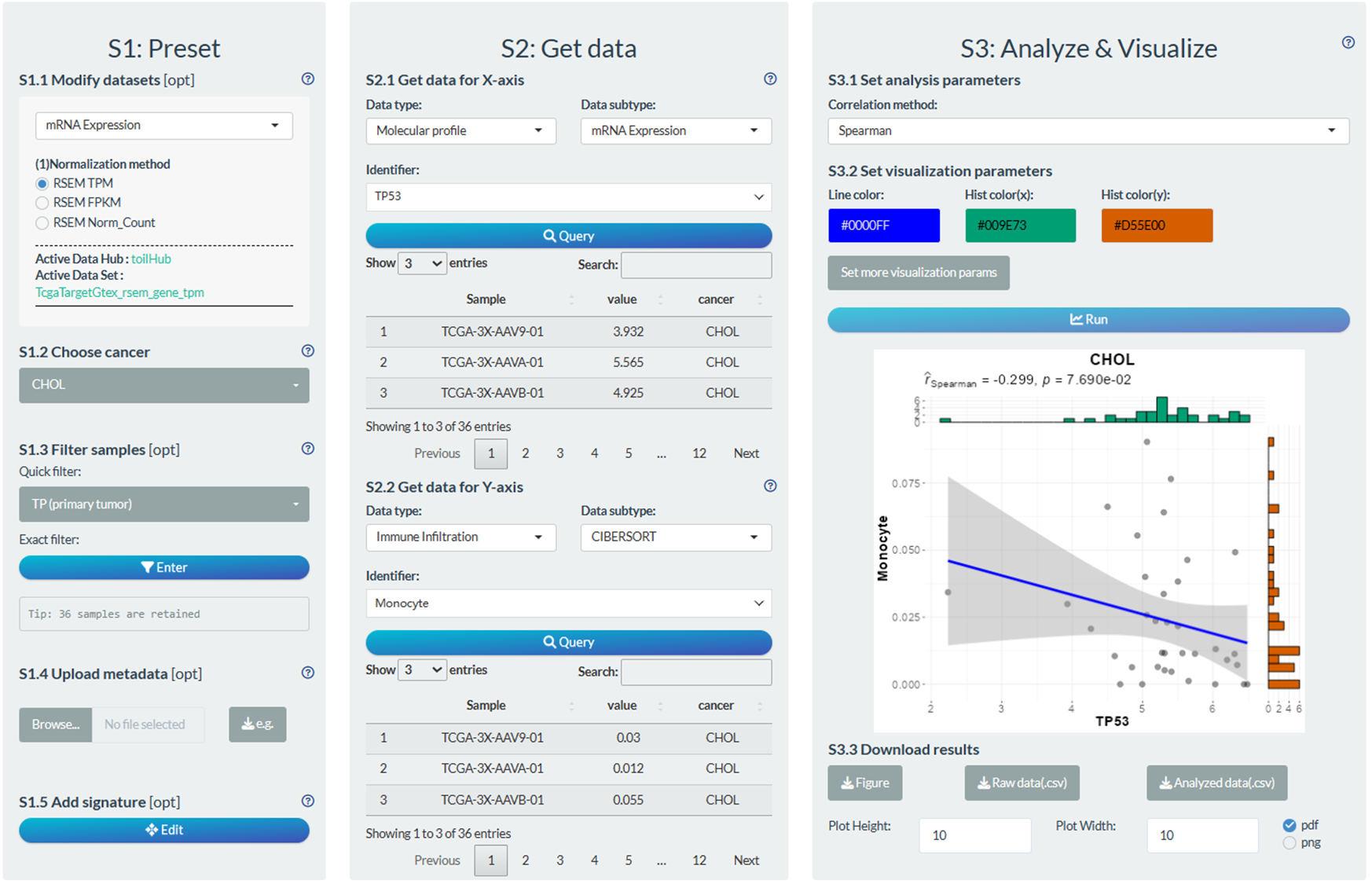
Figure 12.2: Example of correlation analysis in individual mode
12.2.2 Pan-cancer Mode
Perform the correlation analysis between any two identifiers of samples across multiple tumors.
The following is a simple example. (The steps not mentioned in above figure imply default operations.)
S1: Preset
- “S1.1 Modify datasets”: Select the Norm_Count dataset for mRNA Expression dataset.
- “S1.2 Choose cancer”: choose all TCGA cancer types.
- “S1.3 Filter samples”: choose the non-normal samples via the quick filter.
S2: Get data
- “S2.1 Get data for X-axis”: Molecular profile→mRNA Expression→HDAC1
- “S2.2 Get data for Y-axis”: Molecular profile→mRNA Expression→APOE
S3: Analyze & Visualize
- “S3.1 Set analysis parameters”: Pearson
- “S3.2 Set visualization parameters”: Adjust the names of main title and axis title.
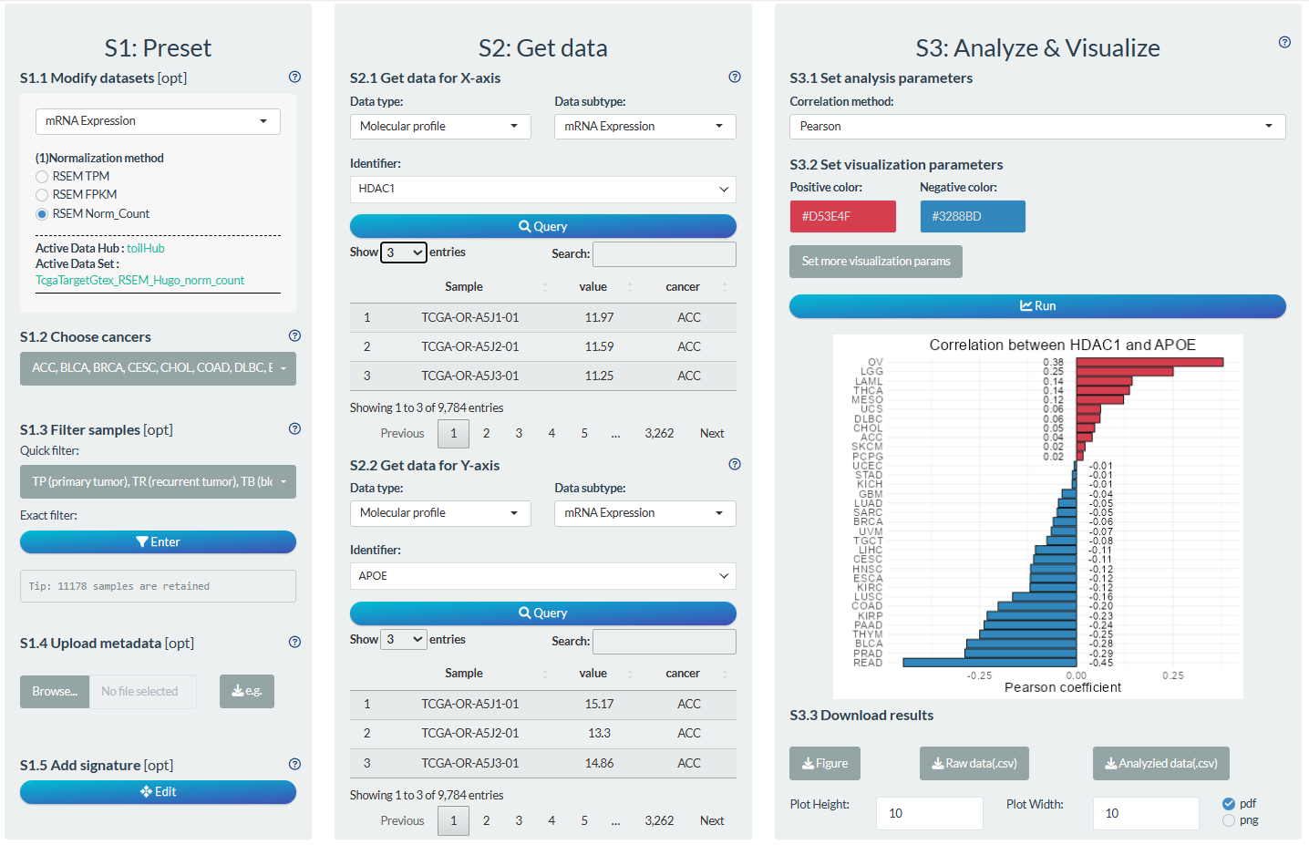
Figure 12.3: Example of correlation analysis in pan-cancer mode
12.2.3 Batch Screen Mode
Perform the correlation analysis between multiple identifiers and one identifier of samples from one tumor.
The following is a simple example. (The steps not mentioned in above figure imply default operations.)
S1: Preset
- “S1.2 Choose cancer”: choose the CHOL (Cholangiocarcinoma) cancer type
- “S1.3 Filter samples”: choose the primary tumor samples via the quick filter.
S2: Get data
- “S2.1 Get batch data for X-axis”: Molecular profile→mRNA Expression→ genes of HALLMARK_APOPTOSIS pathways
- “S2.2 Get data for Y-axis”: Immune Infiltration→CIBERSORT→ Monocyte
S3: Analyze
- “S3.1 Set analysis parameters”: Spearman
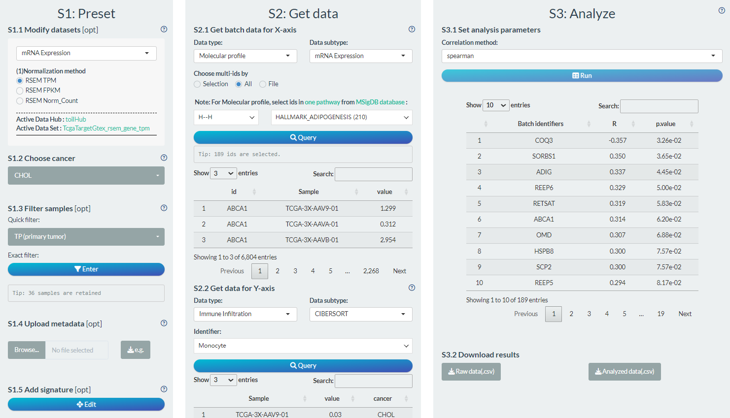
Figure 12.4: Example of correlation analysis in batch screen mode
12.3 Comparison analysis
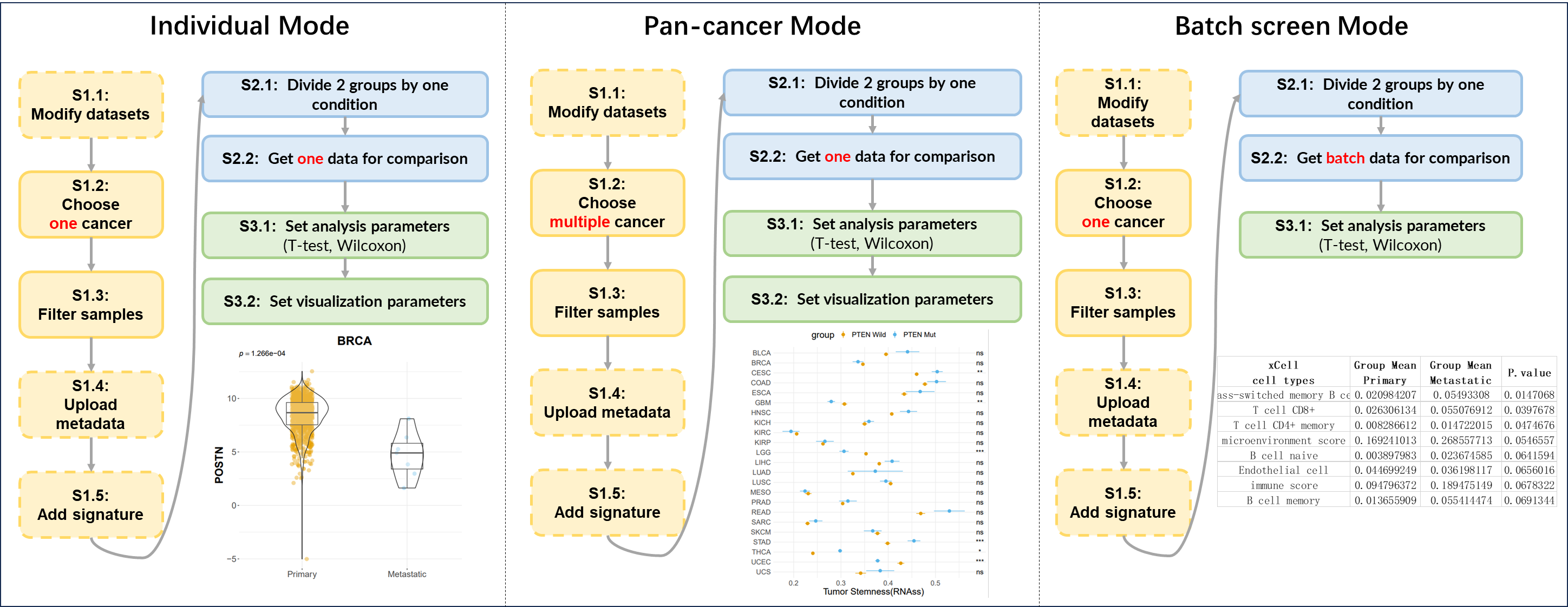
Figure 12.5: 3 modes of comparison analysis
12.3.1 Individual Mode
Perform the comparison analysis of one identifier between two groups of samples from one tumor.
The following is a simple example. (The steps not mentioned in above figure imply default operations.)
S1: Preset
- “S1.2 Choose cancer”: choose the BRCA (Breast invasive carcinoma) cancer type
- “S1.3 Filter samples”: choose the non-normal samples via the quick filter.
S2: Get data
- “S2.1 Divide 2 groups by one condition”: Group1→Primary tumor samples; Group2→Metastatic tumor samples
- “S2.2 Get data for comparison”: Molecular profile→mRNA Expression→POSTN
S3: Analyze & Visualize
- “S3.1 Set analysis parameters”: Wilcoxon test
- “S3.2 Set visualization parameters”: Remove x-axis title.
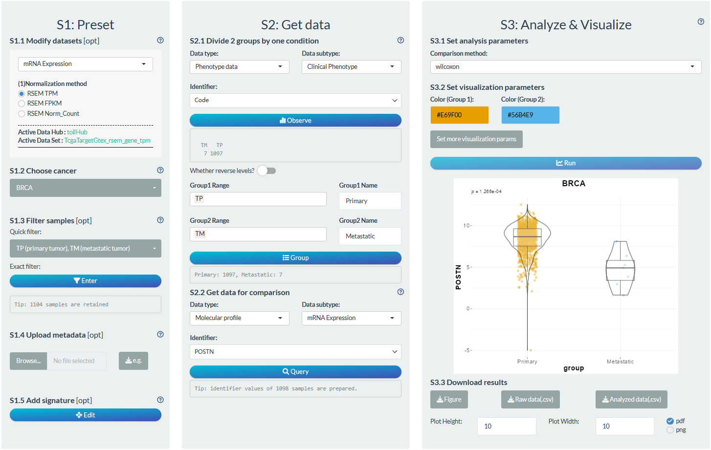
Figure 12.6: Example of comparison analysis in individual mode
12.3.2 Pan-cancer Mode
Perform the comparison analysis of one identifier between two groups of samples across multiple tumors.
The following is a simple example. (The steps not mentioned in above figure imply default operations.)
S1: Preset
- “S1.2 Choose cancer”: choose the all TCGA cancer types.
- “S1.3 Filter samples”: choose the primary tumor samples via the quick filter. Further choose samples with age above 60 via the exact filter.
S2: Get data
- “S2.1 Divide 2 groups by one condition”: Group1→ gene PTEN mutation; Group2→ gene PTEN wild-type.
- “S2.2 Get data for comparison”: Tumor index → Tumor Stemness →RNAss
S3: Analyze & Visualize
- “S3.1 Set analysis parameters”: t-test
- “S3.2 Set visualization parameters”: adjust x-axis title.
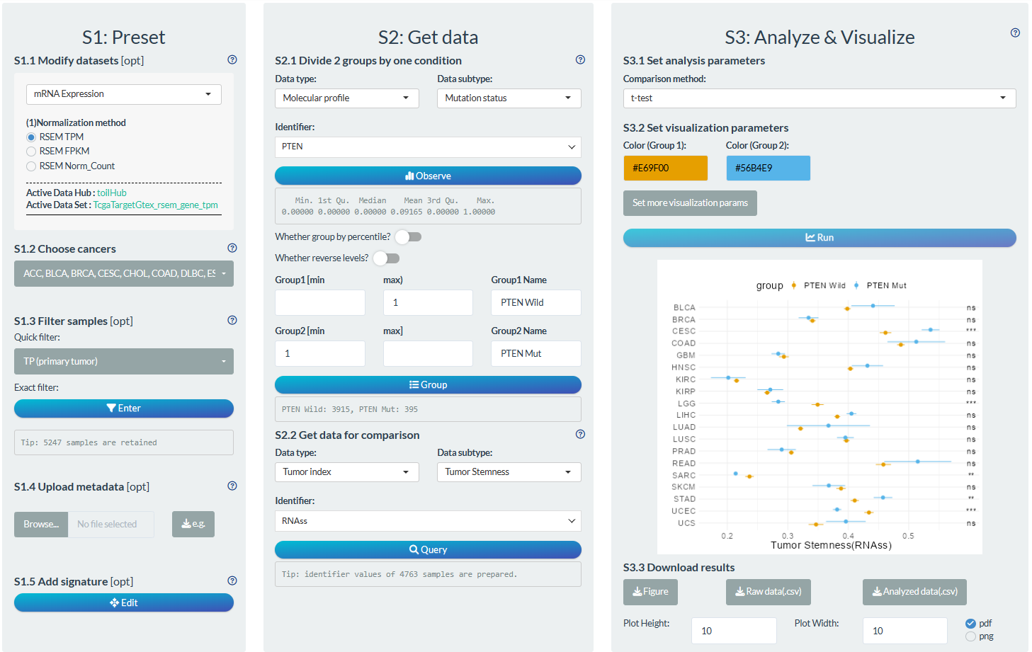
Figure 12.7: Example of comparison analysis in pan-cancer mode
12.3.3 Batch Screen Mode
Perform the comparison analysis of multiple identifier between two groups of samples from one tumor.
The following is a simple example. (The steps not mentioned in above figure imply default operations.)
S1: Preset
- “S1.2 Choose cancer”: choose the BRCA (Breast invasive carcinoma) cancer type
- “S1.3 Filter samples”: choose the non-normal samples via the quick filter.
S2: Get data
- “S2.1 Divide 2 groups by one condition”: Group1→Primary tumor samples; Group2→Metastatic tumor samples
- “S2.2 Get data for comparison”: Immune Infiltration→XCELL→ Monocyte
S3: Analyze
- “S3.1 Set analysis parameters”: Wilcoxon test
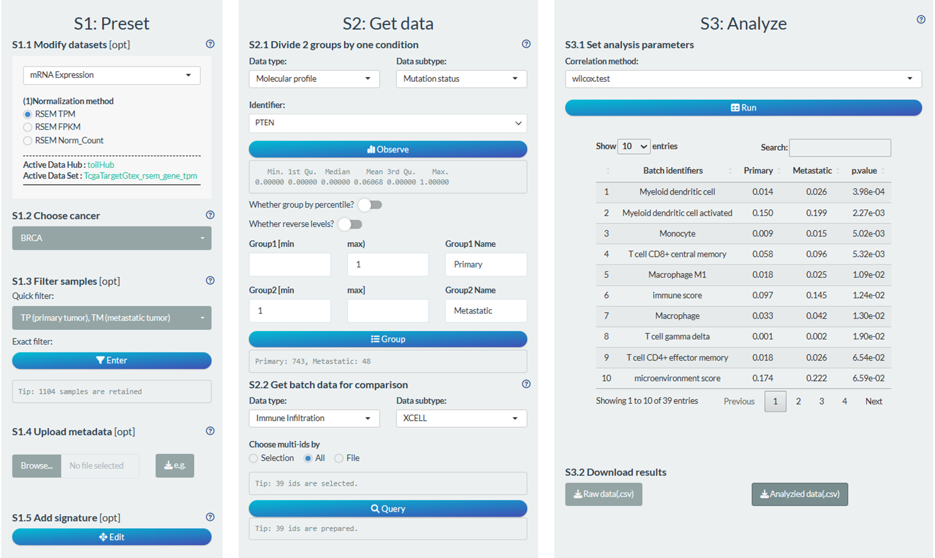
Figure 12.8: Example of comparison analysis in batch screen mode
12.4 Survival analysis
By default, both log-rank and cox regression survival analysis are performed for two groups of samples divided according to one condition. Here, we devised a switch “Whether use initial data before grouping?” at S3.1 steps with following function:
If its status is off , the above default analysis will performed;
If its status is on and the grouping condition is continuous:
- For log-rank test, it will search the optimal cutoff with most significant survival difference;
- For Cox regression, it will directly build the cox model based on the continuous variable.
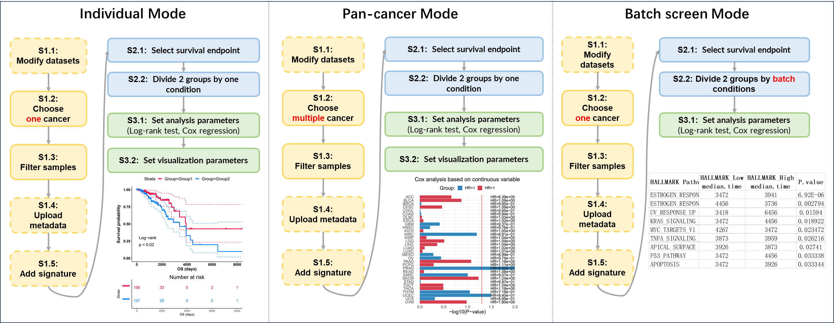
Figure 12.9: 3 modes of survival analysis
12.4.1 Individual Mode
Perform the survival analysis between two groups of samples generated by one identifier from one tumor.
The following is a simple example. (The steps not mentioned in above figure imply default operations.)
S1: Preset
- “S1.1 Modify datasets”: Select the 27K Methylation datasets; Select the cg15206330 site to represent TP53 methylation
- “S1.2 Choose cancer”: choose the BRCA (Breast invasive carcinoma) cancer type
- “S1.3 Filter samples”: choose the non-normal samples via the quick filter.
S2: Get data
- “S2.1 Select survival endpoint”: Select the OS event
- “S2.2 Divide 2 groups by one condition”: Group1: TP53 methylation higher 50%, Group2: TP53 methylation lower 50%
S3: Analyze & Visualize
- “S3.1 Set analysis parameters”: Log-rank text
- “S3.2 Set visualization parameters”: Modify color; Set confidence interval.
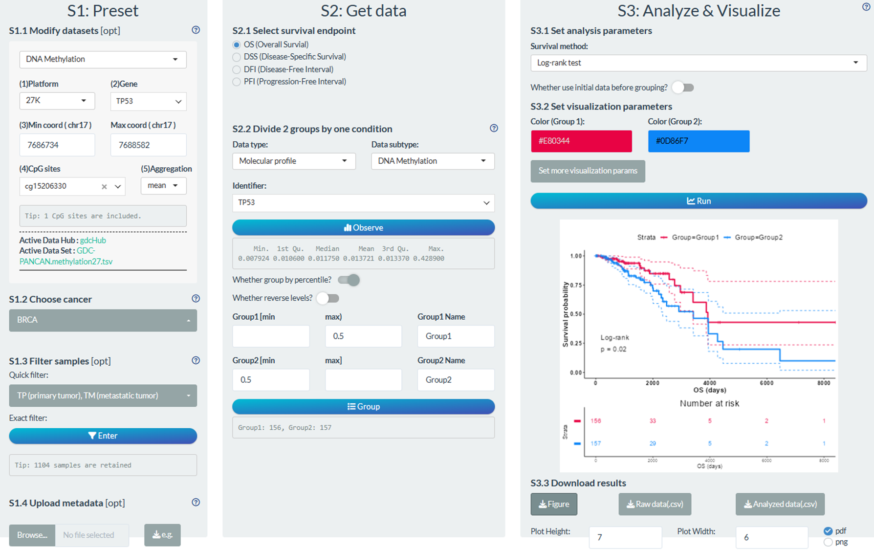
Figure 12.10: Example of survival analysis in individual mode
12.4.2 Pan-cancer Mode
Perform the survival analysis between two groups of samples generated by one identifier across multiple tumor.
The following is a simple example. (The steps not mentioned in above figure imply default operations.)
S1: Preset
- “S1.2 Choose cancer”: choose the BRCA cancer type
- “S1.3 Filter samples”: choose the non-normal samples via the quick filter.
S2: Get data
- “S2.1 Select survival endpoint”: Select the OS event
- “S2.2 Divide 2 groups by one condition”: Group1: Signature value higher 10%, Group2: Signature value lower 10%
S3: Analyze & Visualize
- “S3.1 Set analysis parameters”: Univariate Cox regression; Use the initial data.
- “S3.2 Set visualization parameters”: Add main title.
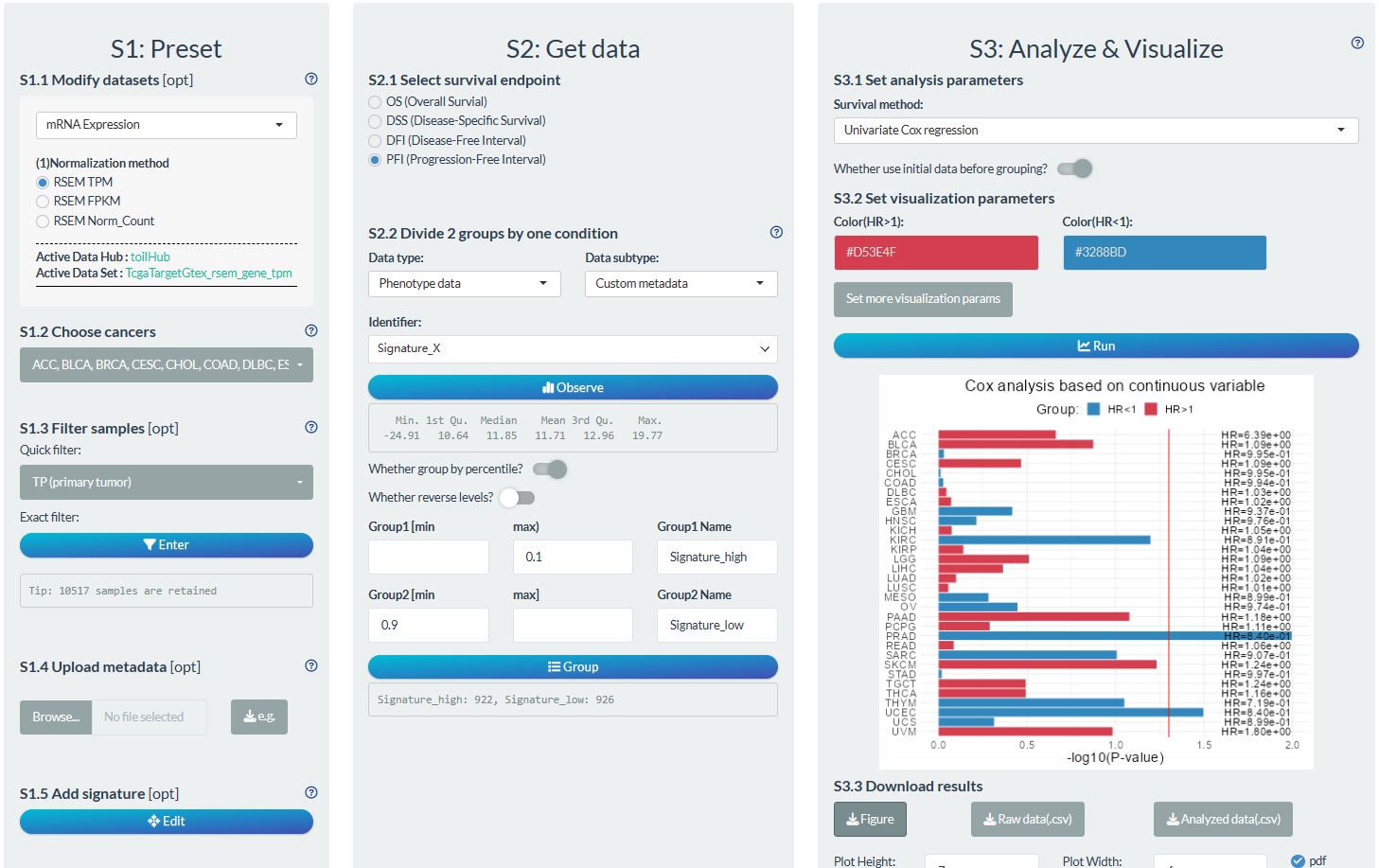
Figure 12.11: Example of survival analysis in pan-cancer mode
12.4.3 Batch Screen Mode
Perform the survival analysis between two groups of samples generated by multiple identifiers from one tumor.
The following is a simple example. (The steps not mentioned in above figure imply default operations.)
S1: Preset
- “S1.2 Choose cancer”: choose the all TCGA cancer types
- “S1.3 Filter samples”: choose the primary tumor samples via the quick filter.
- “S1.5 Add signature”: Design a molecular signature and add to custom metadata.
S2: Get data
- “S2.1 Select survival endpoint”: Select the PFI event
- “S2.2 Divide 2 groups by one condition”: Pathway activity→HALLMARK pathways→Group1: score higher 50%, Group2: score lower 50%
S3: Analyze
- “S3.1 Set analysis parameters”: Log-rank test
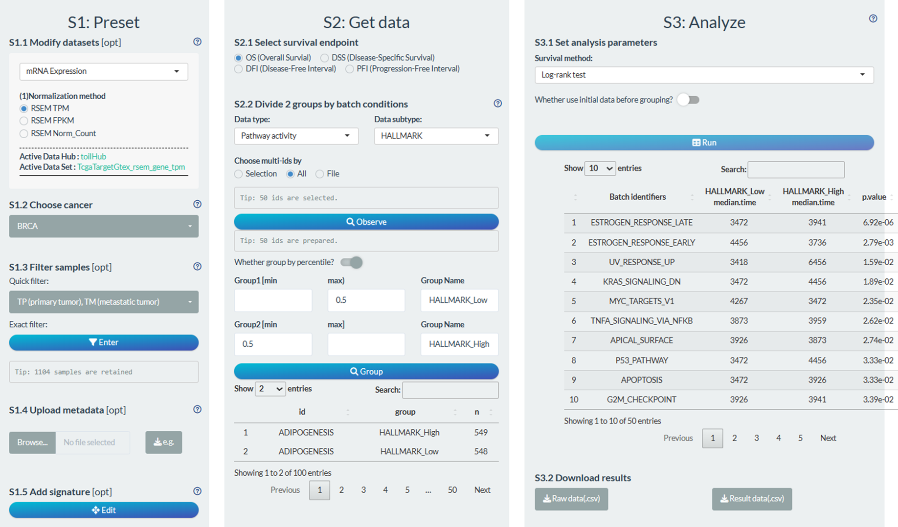
Figure 12.12: Example of survival analysis in batch screen mode
12.5 Cross-Omics analysis
Recently, we have added one pipeline for TCGA cross-omics analysis to simultaneously explore the molecular features of multiple omics across pan-cancers.
12.5.1 Gene Cross-Omics Analysis
Perform the cross-omics analysis at the gene level, involving Gene expression, Gene Mutation, Gene CNV, Transcript expression, DNA methylation.
The following is a simple example. (The steps not mentioned in above figure imply default operations.)
S1: Preset
- “S1.2 Choose cancer”: choose the all TCGA cancer types
- “S1.3 Filter samples”: By default, select all normal samples and tumor samples.
S2: Get data
- “S2.1 Select one gene”: Select gene TP53
- “S2.2 Load mRNA/Mutation/CNV data”: Preload the mRNA/Mutation/CNV data of gene to save time in S3 step.
- “S2.3 Load transcript data”: Select and load several transcript of gene, filter invalid transcripts with null value.
- “S2.4 Load methylation data”: Select several CpG sits of gene and load methyaltion data.
S3: Analyze & Visualize : Analyze multi-omics data and visualize by funkyheatmap package.
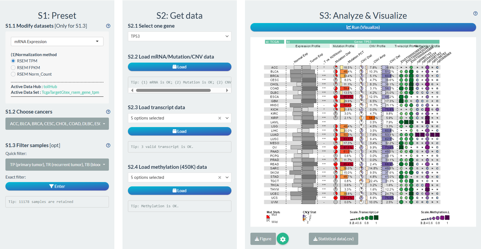
Figure 12.13: Example of Gene Cross-Omics Analysis
Column-1: TCGA Names;
Column-2[Expression Profile]: 0-1 normalized median expression of gene in normal samples (include GTEx);
Column-3[Expression Profile]: 0-1 normalized median expression of gene in tumor samples;
Column-4[Expression Profile]: The significance symbol of gene comparison between tumor and normal samples via Wilcoxon test (P<0.001, “***”; P<0.01, “**”; P<0.05, “*”; P>0.05, “-”).
Column-5[Mutation Profile]: The distribution of gene mutation or wild status in tumor samples.
Column-6[Mutation Profile]: The percentage of gene mutation status in tumor samples.
Column-7[CNV Profile]: The distribution of gene copy number variation status in tumor samples (-2, homozygous deletion; -1, single copy deletion; 0, diploid normal copy; 1: low-level copy number amplification; 2: high-level copy number amplification).
Column-8[CNV Profile]: The percentage of gene copy number amplification (1,2) in tumor samples.
Column-9[CNV Profile]: The percentage of gene copy number deletion (-1, -2) in tumor samples.
Column-Selected transcript(s) of one gene[CNV Profile]: The median transcript expression in tumor samples.
Column-Selected CpG sites of one gene[Methylation Profile]: The median beta value of CpG sites in tumor samples.
12.5.2 Pathway Cross-Omics Analysis
Perform the cross-omics analysis at the pathway level, involving Gene expression, Gene Mutation, Gene CNV.
The following is a simple example. (The steps not mentioned in above figure imply default operations.)
S1: Preset
- “S1.2 Choose cancer”: choose the all TCGA cancer types
- “S1.3 Filter samples”: By default, select all normal samples and tumor samples.
S2: Get data
- “S2.1 one pathway”: Select pathway HALLMARK_ADIPOGENESIS
S3: Analyze & Visualize : Analyze multi-omics data and visualize by funkyheatmap package.
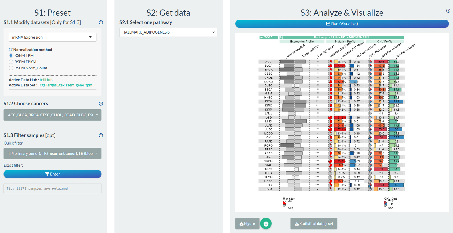
Figure 12.14: Example of Pathway Cross-Omics Analysis
Column-1: TCGA Names;
Column-2[Expression Profile]: 0-1 normalized median ssGSEA score of pathway in normal samples (include GTEx);
Column-3[Expression Profile]: 0-1 normalized median ssGSEA score of gene in tumor samples;
Column-4[Expression Profile]: The significance symbol of gene comparison between tumor and normal samples via Wilcoxon test (P<0.001, “***”; P<0.01, “**”; P<0.05, “*”; P>0.05, “-”).
Column-5[Mutation Profile]: The distribution of mutation or wild pathway gene status in tumor samples. If one of pathway genes is mutated, it is considered as mutation.
Column-6[Mutation Profile]: The percentage of pathway mutation status in tumor samples.
Column-7[Mutation Profile]: The mean counts of mutated pathway genes in tumor samples.
Column-8[CNV Profile]: The distribution of pathway gene copy number variation status in tumor samples. (Amp, homozygous deletion or single copy deletion; Non, diploid normal copy; Del, Copy number amplification.)
Column-9[CNV Profile]: The copy number amplification percentage of pathway genes in tumor samples.
Column-10[CNV Profile]: The copy number deletion percentage of pathway gene in tumor samples.