Chapter 11 TPC Pipelines(1)

11.1 Extensive tumor data

11.1.1 Compiling types of identifiers

1. For TCGA samples, there are 5 main data types and 23 subtypes (except for Custom metadata).

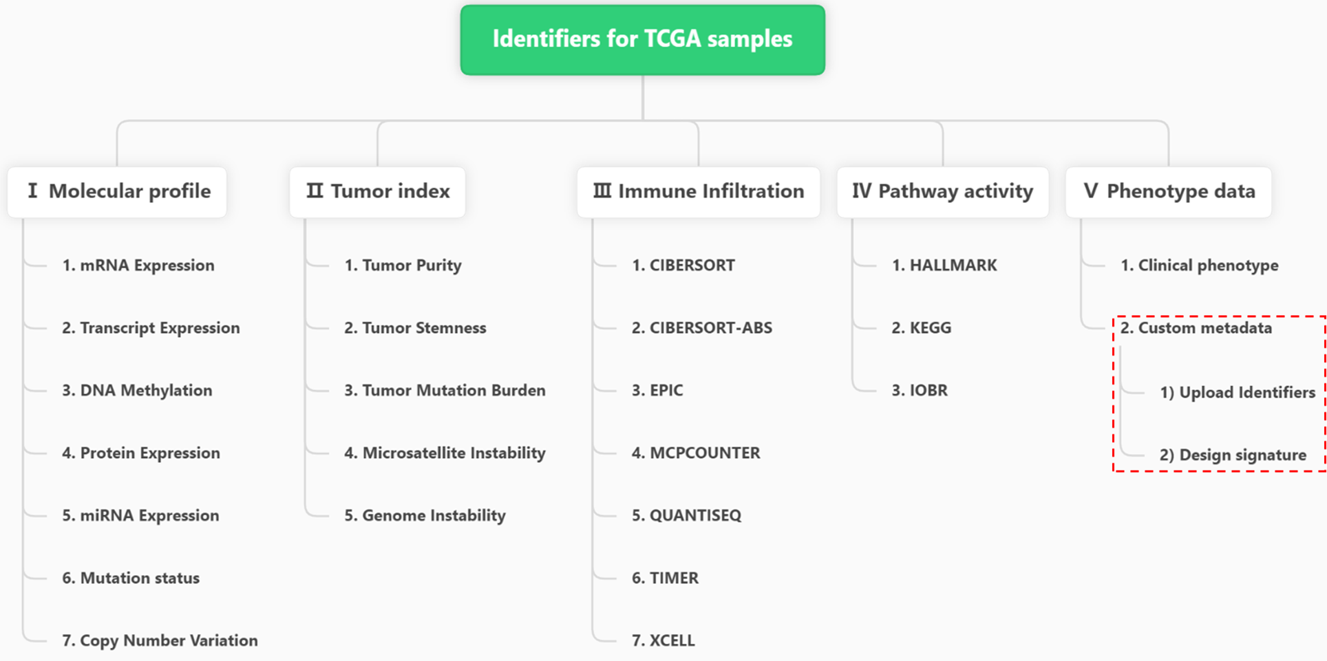
Figure 11.1: Hierarchical types of TCGA Identifiers

2. For PCAWG samples, there are 5 main data types and 17 subtypes (except for Custom metadata).

3. For CCLE samples, there are 3 main data types and 6 subtypes (except for Custom metadata).

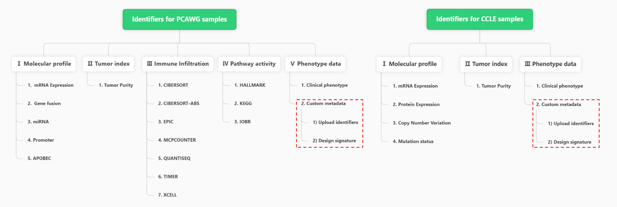
Figure 11.2: Hierarchical types of PCAWG and CCLE Identifiers

About the core data type —— Molecular profile, the initial step of all analysis pipelines involves the check and modification of molecular datasets through the Modify datasets[opt] widget. For some molecular types of TPC databases, there are alternative datasets for users to select, which greatly enriches the analytical possibilities

• Among the 7 types of TCGA molecules, 4 of them have the alternative datasets.

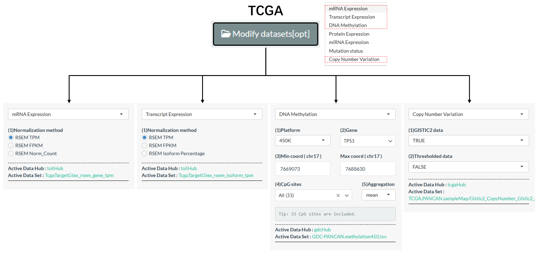
Figure 11.3: Alternative datasets of TCGA molecules

Tips: For DNA Methylation, mean value of all CpG sites under one gene will be calculated for the gene by default. In the Modify datasets[opt] widget, users can furtherly limit its CpG sites and modify the aggregation method (e.g. median).

• Among the 5 types of PCAWG molecules, 2 of them have the alternative datasets.

• Among the 4 types of CCLE molecules, 1 of them has the alternative datasets.

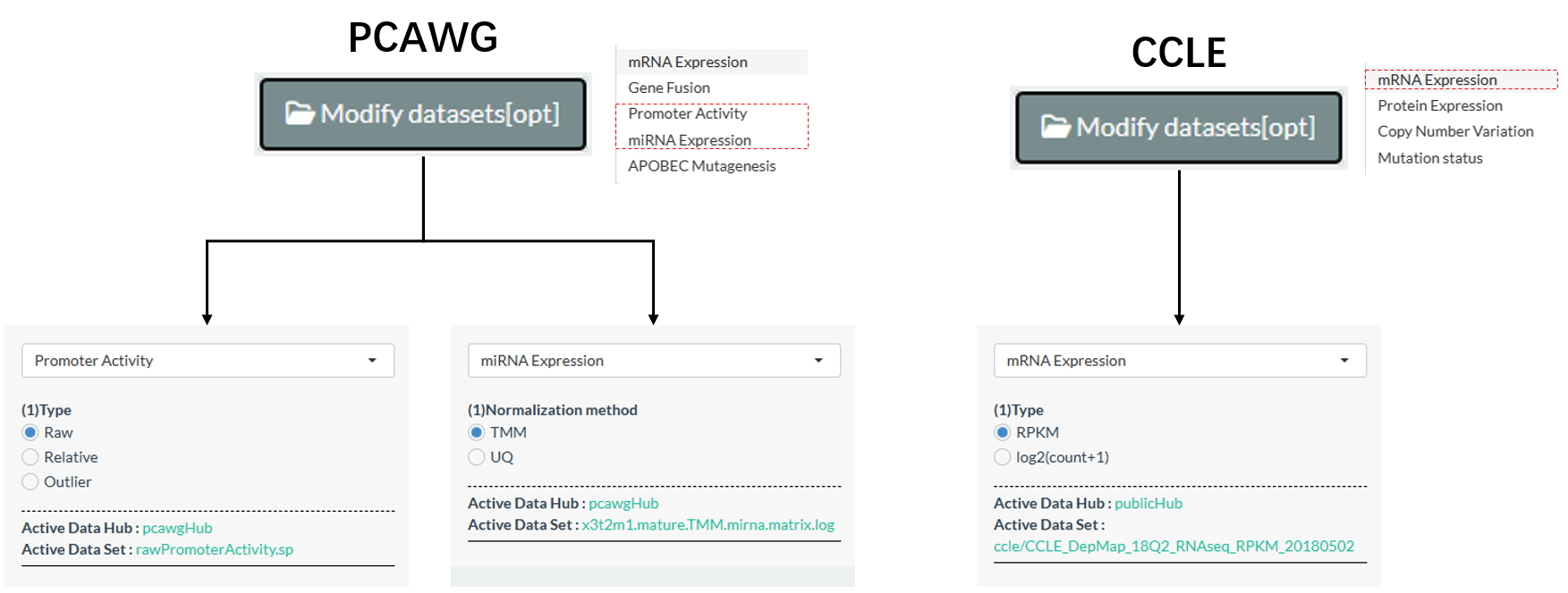
Figure 11.4: Alternative datasets of PCAWG and CCLE molecules

11.1.2 Reference of full identifiers

• In the “Help→ID query” page, all identifiers for “Molecular profile”, “Tumor index”, “Immune Infiltration”, “Pathway activity”, “Phenotype data” types of TPC samples are compiling for easy query before analysis.
• For example, valid identifiers under the TCGA mRNA Expression subtype are shown in the following figure.

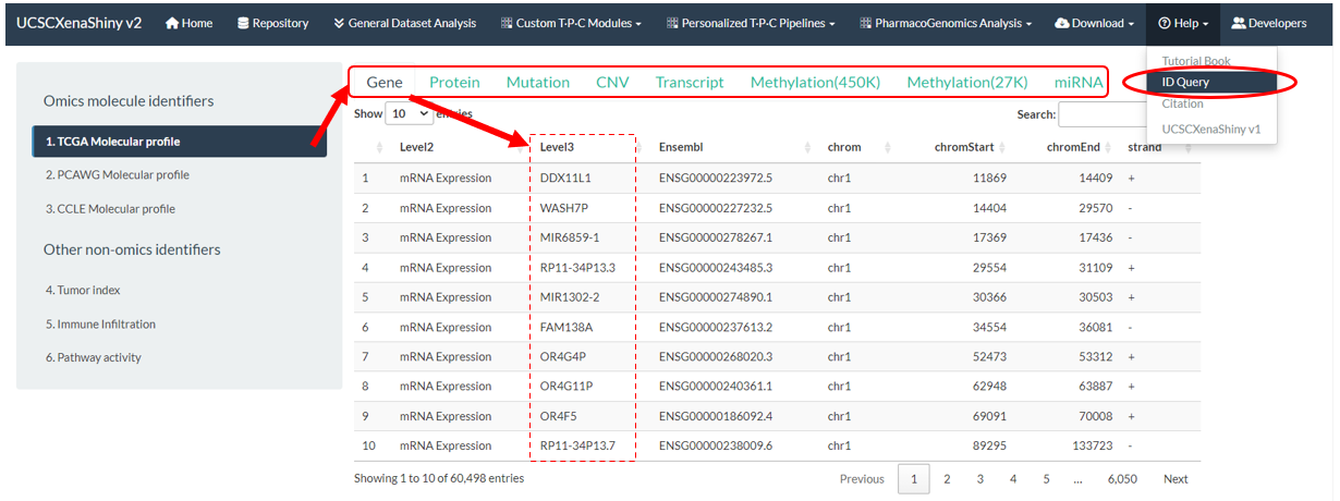
Figure 11.5: TPC Identifiers Query Page

11.1.3 User-defined identifiers

11.1.3.1 Upload of random identifiers

1. Users are enabled to upload random identifiers for joint analysis in the “Upload metadata” part of S1 step.
2. The example file can be downloaded via the right button to see the format requirements.
   • .CSV file;
   • The first column names “Sample” with sample ids (e.g. “TCGA-OR-A5J1-01” for TCGA samples). Only the intersected samples between this column and all TPC samples are considered;
   • The other columns are random identifiers with continuous or categorical values.
3. Upon successful identifiers upload, they will be added into the “Custom metadata” subtype of “Phenotype data”.

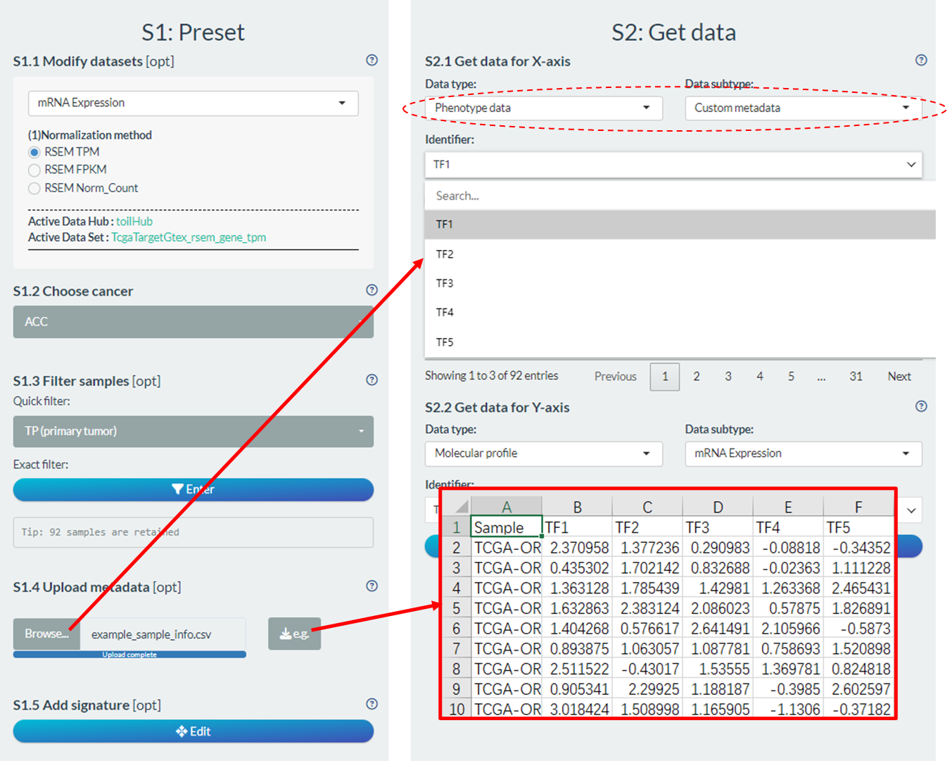
Figure 11.6: Upload of random identifiers

11.1.3.2 Design of custom signature

1. Users can also design custom signature score based on self-defined molecular formula in the “Add signature” part of S1 step.
2. Upon successful signature design and score calculation, they will also be added into the “Custom metadata” subtype of “Phenotype data”.

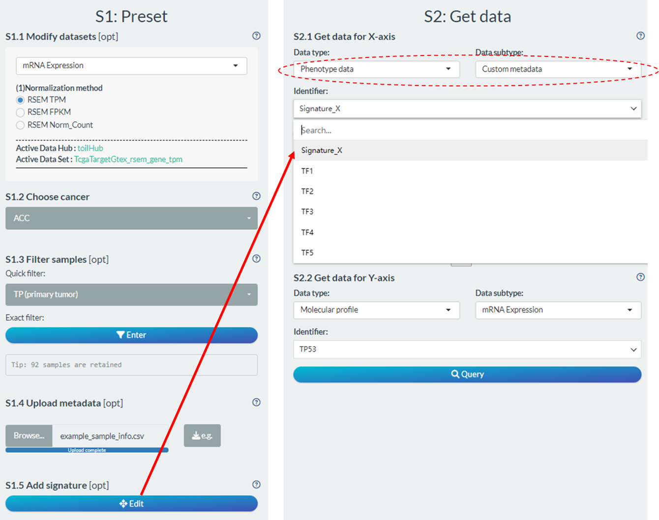
Figure 11.7: Design of custom signature

3. As shown in the figure below, the signature can be set as following steps after clicking Edit button.

• Firstly, modify the name and select the molecular type;
• Then, design the molecular formula comprised of multiple molecules with respective coefficients;
  • The coefficient of each molecule is divided into two parts (Directions and Absolute Coef).
  • The “Del” button will cancel the last set molecule and the “Reset” button will undo all selected molecules.
  • The real-time formula is shown in the bottom.
• Finally, click the “Query data” button to calculate the signature scores and click the right button to add the signature into the “Custom metadata” subtype of “Phenotype data”. In addition, user can obtain the result locally via the bottom button.

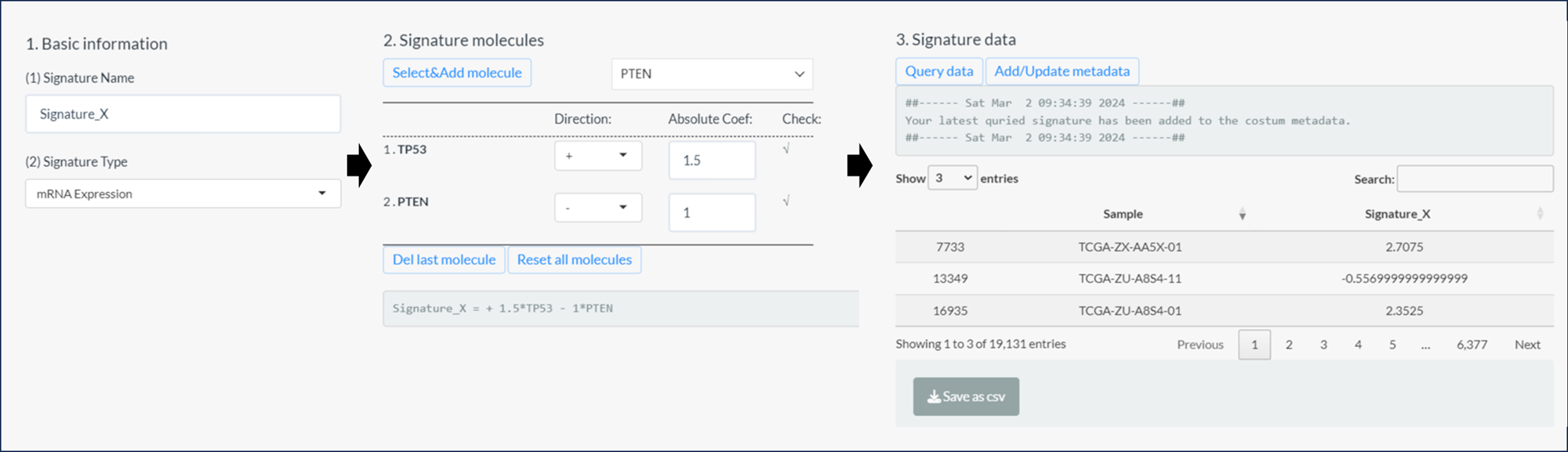
Figure 11.8: 3 steps of signature design

11.2 Sample processing

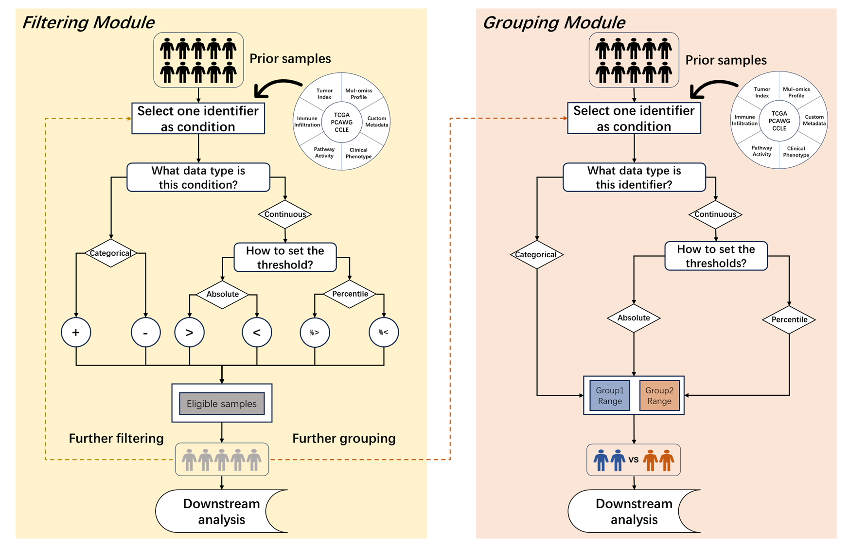
Figure 11.9: Sample filtering and grouping modules

11.2.1 Sample filtering

After selecting one tumor, all its samples will be selected by default. Here, we provide two methods to obtain specific subpopulation in the “Filter samples” part of S1 step.

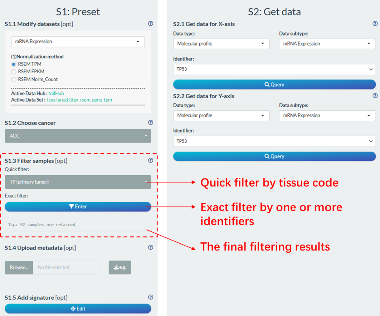
Figure 11.10: Sample filtering module

11.2.1.1 Quick filter

Users can directly make quick selections based on tissue code (pathological) types of samples. Based on the 14th to 15th characters of the TCGA sample ID (e.g., TCGA-19-1787-01), samples can be categorized into different types. The common code types involved in UCSCXenaShiny analysis are shown in the following table.

Code	Definition	Short Letter Code
01	Primary Solid Tumor	TP
02	Recurrent Solid Tumor	TR
03	Primary Blood Derived Cancer - Peripheral Blood	TB
05	Additional - New Primary	TAP
06	Metastatic	TM
07	Additional Metastatic	TAM
11	Solid Tissue Normal	NT

For PCAWG database, you can perform similar operation to quickly select tumor or normal samples. For CCLE database, there is no quick filter.

11.2.1.2 Exact filter

Through this module, users are enabled to perform personalized sample filtering. This followings are operational steps:

1. Set the candidate conditions from comprehensive identifiers. Each addition will rename the selected identifier as “Condition_Num”.
   • When selecting molecular identifier as condition, it may take some time to download from the USCS Xena, depending on the network.
   • For TPC samples, some basic clinical variables have been selected into the candidate pool. For TCGA samples, they include Age, Code, Gender, Stage_ajcc, Stage_clinical, Grade.
2. Get an overview of the distribution of each candidate condition for clear filtering .
   • For continuous variables, the mean and the distribution of multiple percentiles are displayed.
   • For categorical variables, the frequency of each category is displayed.
3. Perform filtering operation based on one or multiple conditions from the above candidate list. Total 6 operators are devised for versatile filtering give the type of each condition.
   • For categorical variable, “+” and “-” are used for retain or discard specific categories of samples.
   • For continuous variable, “>” and “<” are used to set absolute cutoff, while “%>” and “%<” are used to set percentile cutoff.

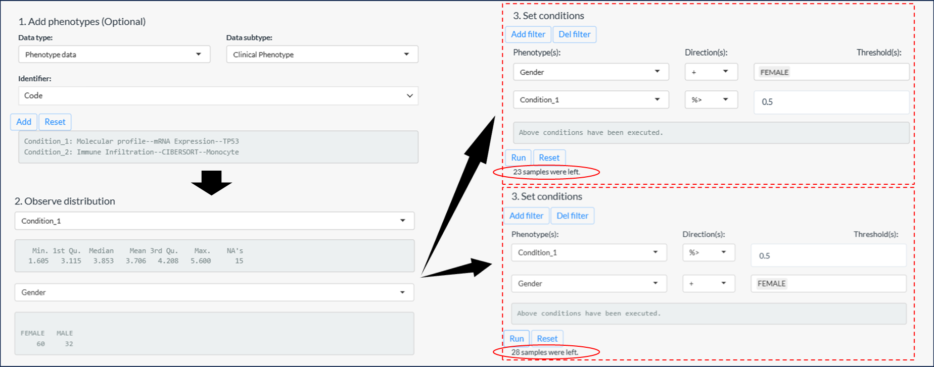
Figure 11.11: 3 steps of sample filtering

Tips: If the percentile cutoff is involved, the results may vary based on the order of filtering, as illustrated in the example above figure.

• The first instance: Samples with the top 50% high expression of TP53 in female samples. → 23 samples
• The second instance: Females from the top 50% of samples with high TP53 expression. → 28 samples

11.2.2 Sample grouping

For binary comparison or survival analysis, it is necessary to divide the samples into two groups based on one specific condition. Here, we also provide a personalized grouping module to flexibly set two ranges of sample populations.

Generally, it has the two main steps:

1. Select one condition and observe its distribution. Similar to the filtering module, it can bring a clear pre-knowledge by observing the distribution of one continuous or categorical condition.

2. Set two non-overlapping sample ranges to group.

• For categorical variable, assign one or more classifications for both groups (Left figure)
• For continuous variable, set the minimum and max thresholds for both group.
  • By default, the first group (Group1) has lower value with left close and right open range, e.g. [0, 1). If its left range is blank, it will represent the minimum value of the condition.
  • And, the second group (Group2) has larger value with left close and right close range, e.g. [0, 1]. If its right range is blank, it will represent the maximum value of the condition.
  • The thresholds can be percentile values (Middle figure) or absolute values (Right figure) depending on purposes.

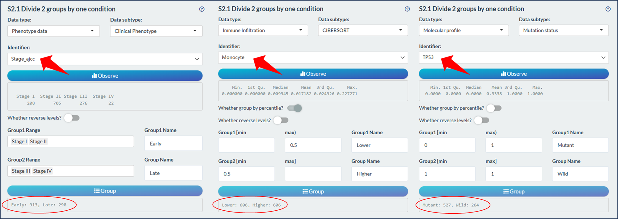
Figure 11.12: Sample grouping module

Tips: By default, the Group1 has the prior order during analysis and visualization. You can click the switch “Whether reverse levels” to change the order.

11.3 Data fetch

After sample selection and processing, we usually need to fetch data for downstream analysis.

11.3.1 Single data

Most of time, we just need to select one identifier and fetch its values. According to the hierarchical organization (Data type → Data subtype → Identifier), select one interesting identifier and then click the “Query button” to fetch data. It’s worth noting that, for Molecular profile data types, it may take some time to download from the UCSC Xena, depending on the network.

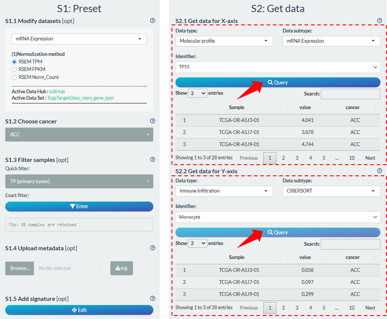
Figure 11.13: Fetch single data

11.3.2 Multiple data

For batch analysis, we can select multiple identifiers based on one of three ways.

1. In the first way (Left figure), user can select batch identifiers of one specific subtype one by one.
2. In the second way (Middle figure), user can select all identifiers of one specific subtype. Notably, for some molecular types with much identifiers, all the identifiers (gene/transcript) belong to one MSigDB signature can be selected.

• These molecular types are “mRNA Expression”, “DNA Methylation”, “Mutation status”, “Copy Number Variation”, “Transcript Expression”.
• The MSigDB gene signatures are obtained via msigdbr package, which can be 9 main categories (bottom table).
• Two links are available for detailed information of selected signature and MSigDB database.

3. In the third way (Right figure), user can directly upload an identifier file with following requirements:

• TXT format;
• One column without colname;
• Only the valid identifiers that overlapped with the selected data subtype are retained

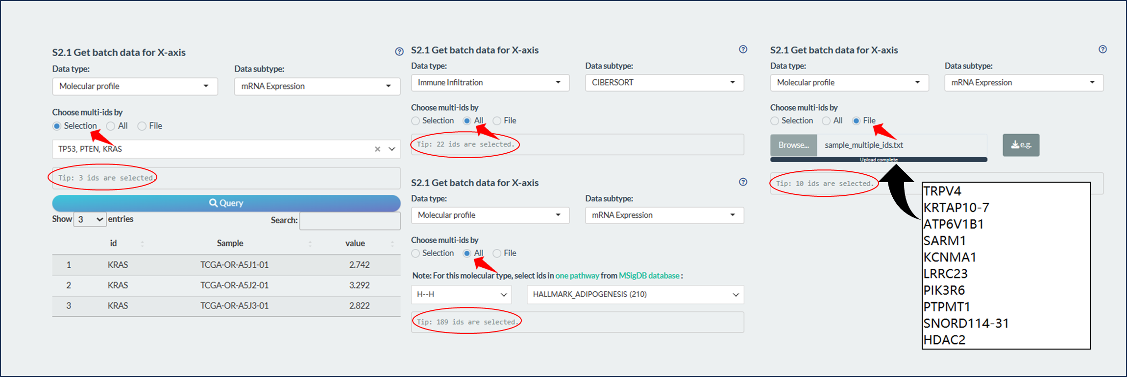
Figure 11.14: Fetch multiple data

---

Category	Notes	Subcategory
H	hallmark gene sets	/
C1	positional gene sets	/
C2	curated gene sets	CGP, CP, CP:BIOCARTA, CP:KEGG, CP:PID, CP:REACTOME, CP:WIKIPATHWAYS
C3	regulatory target gene sets	MIR:MIRDB, MIR:MIR_Legacy, TFT:GTRD, TFT:TFT_Legacy
C4	computational gene sets	CGN, CM
C5	ontology gene sets	GO:BP, GO:CC, GO:MF, HPO
C6	oncogenic signature gene sets	/
C7	immunologic signature gene sets	IMMUNESIGDB, VAX
C8	cell type signature gene sets	/