Chapter 10 TPC Modules
In the “Custom TPC modules” page, there are totally 10 series of modules to quickly explore TPC (TCGA, PCAWG, CCLE) datasets with easy steps, based on the functions introduced in Chapter 5.
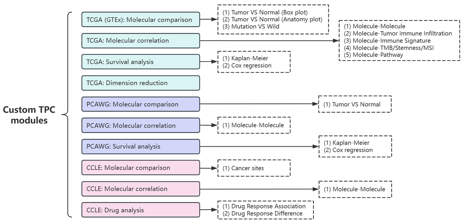
Figure 10.1: All Custom TPC modules in shiny app
10.1 TCGA
| Database | Type | Module |
|---|---|---|
| TCGA | Comparison | Tumor VS Normal (Box plot) |
| TCGA | Comparison | Tumor VS Normal (Anatomy plot) |
| TCGA | Comparison | Mutation VS Wild |
| TCGA | Correlation | Molecule-Molecule |
| TCGA | Correlation | Molecule-Tumor Immune Infiltration |
| TCGA | Correlation | Molecule-Immune Signature |
| TCGA | Correlation | Molecule-TMB/Stemness/MSI |
| TCGA | Correlation | Molecule-Pathway |
| TCGA | Survival | Kaplan-Meier |
| TCGA | Survival | Cox regression |
| TCGA | Dimension Reduction | Dimension reduction |
10.1.1 Comparison
10.1.1.1 TCGA Tumor VS Normal (Box plot)
Compare molecular values between tumor and normal samples combing TCGA and GTEx datasets based on vis_toil_TvsN() and vis_toil_TvsN_cancer() functions.
- Left panel
- Select one of supported multi-omics types;
- Select an identifier or define a signature;
- Select the mode: Pan-cancer or Single-Cancer (For the latter, one tumor type needs to be specified);
- Decide that Whether to include normal samples from GTEx;
- Click the “Go!” button
- Right panel
- Observe the visualization plot of analytical result;
- Pull the sidebar to adjust plot parameters or download results through the top-right widget.
Figure 10.2: The layout of module “Tumor VS Normal (Box plot)”
10.1.1.2 TCGA Tumor VS Normal (Anatomy plot)
Observe the difference of molecular values between pan-cancer tumor and normal samples based on vis_pancan_anatomy() functions.
- Left panel
- Select one of supported multi-omics types;
- Select an identifier or define a signature;
- Click the “Go!” button
- Right panel
- Observe the anatomy plot of analytical result;
- Pull the sidebar to adjust plot parameters or download results through the top-right widget.
Figure 10.3: The layout of module “Tumor VS Normal (Anatomy plot)”
10.1.1.3 TCGA Mutation VS Wild
Compare molecular values between gene-mutant and gene-wild tumor samples based on vis_toil_Mut() and vis_toil_Mut_cancer() functions.
- Left panel
- Select one of supported multi-omics types;
- Select an identifier or define a signature to be compared;
- Select one gene and group according to its mutation status;
- Select the mode: Pan-cancer or Single-Cancer (For the latter, one tumor type needs to be specified);
- Click the “Go!” button
- Right panel
- Observe the visualization plot of analytical result;
- Pull the sidebar to adjust plot parameters or download results through the top-right widget.
Figure 10.4: The steps of module “Mutation VS Wild”
10.1.2 Correlation
10.1.2.1 TCGA Molecule-Molecule
Compute and visualize the correlation between two molecules of tumor samples based on vis_gene_cor() and vis_gene_cor_cancer() functions.
- Left panel
- Select two respective omics types;
- Select two specific identifiers as X-axis and Y-axis;
- Select one or more TCGA types;
- Select correlation method;
- Decide that whether the correlation is corrected based on tumor purity;
- Click the “Go!” button.
- Right panel
- Observe the scatter plot of analytical result;
- Pull the sidebar to adjust plot parameters or download results through the top-right widget.
Figure 10.5: The steps of module “Molecule-Molecule”
10.1.2.2 TCGA Molecule-Tumor Immune Infiltration
Compute the correlation of pan-cancers between one molecule and tumor immune infiltration of pan-cancer samples based on vis_gene_TIL_cor() function.
- Left panel
- Select one of supported multi-omics types;
- Select an identifier or define a signature;
- Select multiple TIL estimation;
- Select correlation method;
- Click the “Go!” button.
- Right panel
- Observe the heatmap plot of analytical result;
- Pull the sidebar to adjust plot parameters or download results through the top-right widget.
Figure 10.6: The steps of module “Molecule-Tumor Immune Infiltration”
10.1.2.3 TCGA Molecule-Immune Signature
Compute the correlation of pan-cancers between one molecule and tumor Immune Signature based on vis_gene_immune_cor() function.
- Left panel
- Select one of supported multi-omics types;
- Select an identifier or define a signature;
- Select one category of immune cell type scores;
- Select correlation method;
- Click the “Go!” button.
- Right panel
- Observe the heatmap plot of analytical result;
- Pull the sidebar to adjust plot parameters or download results through the top-right widget.
Figure 10.7: The steps of module “Molecule-Immune Signature”
10.1.2.4 TCGA Molecule-TMB/Stemness/MSI
Compute the correlation of pan-cancers between one molecule and TMB/Stemness/MSI index based on vis_gene_tmb_cor(), vis_gene_msi_cor() and vis_gene_stemness_cor() functions.
- Left panel
- Select one of supported multi-omics types;
- Select an identifier or define a signature;
- Select one of collected tumor index;
- Select correlation method;
- Click the “Go!” button.
- Right panel
- Observe the radar plot of analytical result;
- Pull the sidebar to adjust plot parameters or download results through the top-right widget.
Figure 10.8: The steps of module “Molecule-TMB/Stemness/MSI”
10.1.2.5 TCGA Molecule-Pathway
Compute the correlation of between one molecule and pathway score of tumor samples based on vis_gene_pw_cor() function.
- Left panel
- Select one of supported multi-omics types;
- Select an identifier or define a signature;
- Select one of calculated pathway scores (ssGSEA);
- Select correlation method;
- Click the “Go!” button.
- Right panel
- Observe the scatter plot of analytical result;
- Pull the sidebar to adjust plot parameters or download results through the top-right widget.
Figure 10.9: The steps of module “Molecule-Pathway”
10.1.3 Survival analysis
10.1.3.1 TCGA Kaplan-Meier
Perform one molecular Log-rank survival analysis based on tcga_surv_plot() function.
- Left panel
- Select one of supported multi-omics types;
- Select an identifier or define a signature;
- Select one TCGA cancer and select one endpoint as survival event;
- Filter samples by Gender, Age, Stage;
- Select the grouping method;
- Click the “Go!” button.
- Right panel
- Observe the survival curves of analytical result;
- Pull the sidebar to adjust plot parameters or download results through the top-right widget.
Figure 10.10: The steps of module “Kaplan-Meier”
10.1.3.2 TCGA Cox regression
Perform one molecular Log-rank survival analysis across pan-cancers based on vis_unicox_tree() function.
- Left panel
- Select one of supported multi-omics types;
- Select an identifier or define a signature;
- Select one endpoint as survival event;
- Click the “Go!” button.
- Right panel
- Observe the forest plot of analytical result;
- Pull the sidebar to adjust plot parameters or download results through the top-right widget.
Figure 10.11: The steps of module “Cox regression”
10.1.4 Dimension Reduction
10.1.4.1 TCGA Dimension reduction
Perform molecular dimension reduction analysis based on vis_dim_dist() function.
- Left panel
- Select one of supported multi-omics types;
- Select multiple identifiers via one of three ways, then click the “Cache data” button;
- “Select”: One-by-one selection;
- “Pathway”: batch selection under one pathway;
- “File”: Upload of identifier file.
- Set the sample range and grouping;
- “Preset Group”: select one or more TCGA cancers and one clinical phenotype as grouping criteria.
- “Custom Group”: upload files with custom samples and group columns. See details by downloading example file.
- Select the algorithm of dimension reduction;
- Click the “Go!” button.
- Right panel
- Observe the scatter plot of analytical result;
- Pull the sidebar to adjust plot parameters or download results through the top-right widget.
Figure 10.12: The steps of module “Dimension reduction”
10.2 PCAWG
| Database | Type | Module |
|---|---|---|
| PCAWG | Comparison | Tumor VS Normal |
| PCAWG | Correlation | Molecule-Molecule |
| PCAWG | Survival | Kaplan-Meier |
| PCAWG | Survival | Cox regression |
10.2.1 Comparison analysis
10.2.1.1 PCAWG Tumor VS Normal
Compare molecular values between tumor and normal samples of PCAWG projects based on vis_pcawg_dist() function.
- Left panel
- Select one of supported multi-omics types;
- Select an identifier or define a signature;
- Click the “Go!” button.
- Right panel
- Observe the visualization plot of analytical result (Some of projects only have tumor samples);
- Pull the sidebar to adjust plot parameters or download results through the top-right widget.
Figure 10.13: The steps of module “Tumor VS Normal”
10.2.2 Correlation analysis
10.2.2.1 PCAWG Molecule-Molecule
Compute and visualize the correlation between two molecules based on vis_pcawg_gene_cor() function.
- Left panel
- Select two respective omics types;
- Select two specific identifiers as X-axis and Y-axis;
- Select one or more PCAWG projects;
- Select correlation method;
- Decide that whether the correlation is corrected based on tumor purity;
- Click the “Go!” button.
- Right panel
- Observe the scatter plot of analytical result;
- Pull the sidebar to adjust plot parameters or download results through the top-right widget.
<img src=“images/p1115.png” alt=“The steps of module”Molecule-Molecule”” width=“100%” />
Figure 10.14: The steps of module “Molecule-Molecule”
10.2.3 Survival analysis
Notes: Only OS endpoint for PCAWG samples.
10.2.3.1 PCAWG Kaplan-Meier
Perform one molecular Log-rank survival analysis in one PCAWG project.
- Left panel
- Select one of supported multi-omics types;
- Select an identifier or define a signature;
- Select one PCAWG project;
- Filter samples by Gender, Age;
- Select the grouping method;
- Click the “Go!” button.
- Right panel
- Observe the survival curves of analytical result;
- Pull the sidebar to adjust plot parameters or download results through the top-right widget.
Figure 10.15: The steps of module “Kaplan-Meier”
10.2.3.2 PCAWG Cox regression
Perform one molecular Log-rank survival analysis in All PCAWG projects based on vis_pcawg_unicox_tree() function.
- Left panel
- Select one of supported multi-omics types;
- Select an identifier or define a signature;
- Click the “Go!” button.
- Right panel
- Observe the forest plot of analytical result;
- Pull the sidebar to adjust plot parameters or download results through the top-right widget.
Figure 10.16: The steps of module “Cox regression”
10.3 CCLE
| Database | Type | Module |
|---|---|---|
| CCLE | Comparison | Cancer Primary Sites |
| CCLE | Correlation | Molecule-Molecule |
10.3.1 Comparison analysis
10.3.1.1 CCLE Cancer Primary Sites
Compare molecular values of cancer cell lines from different primary site based on vis_ccle_tpm() function.
- Left panel
- Select one of supported multi-omics types;
- Select an identifier or define a signature;
- Click the “Go!” button.
- Right panel
- Observe the visualization plot of analytical result;
- Pull the sidebar to adjust plot parameters or download results through the top-right widget.
Figure 10.17: The steps of module “Cancer Primary Sites”
10.3.2 Correlation analysis
10.3.2.1 CCLE Molecule-Molecule
Compute and visualize the correlation between two molecules based on CCLE database based on vis_ccle_gene_cor() function.
- Left panel
- Select two respective omics types;
- Select two specific identifiers as X-axis and Y-axis;
- Select one or more primary sites;
- Select correlation method;
- Click the “Go!” button.
- Right panel
- Observe the scatter plot of analytical result;
- Pull the sidebar to adjust plot parameters or download results through the top-right widget.
Figure 10.18: The steps of module “Molecule-Molecule”