Recently, we have added some new modules for general TCGA data analysis and visualization. Here, we will provide the tutorials for easy use. Please note it is not the latest version and we are still in the stage of development. Therefore, if you have any question, please do not hesitate to contact us on GitHub or email (lishensuo@163.com) which could greatly contribute to UCSCXenaShiny V2.0 process.
The temporary tutorial is based on the latest commit On November 18, 2023. It may be outdated in the future and we will update the latest tutorials as soon as possible.
0 Prior knowledge
- Paper: UCSCXenaShiny: An R/CRAN Package for Interactive Analysis of UCSC Xena Data, Bioinformatics, 2021;, btab561, https://doi.org/10.1093/bioinformatics/btab561.
- GitHub: https://github.com/openbiox/UCSCXenaShiny
- Website: https://shiny.hiplot.cn/ucsc-xena-shiny/
1. key features
For the general exploration of TCGA data, we support the following key features.
- 3 analysis methods: (1) Correlation; (2) Comparison; (3) Survival analysis.
- 3 analysis modes: (1) One data on one cancer; (2) One data on multiple cancers; (3) Multiple data on one cancer.
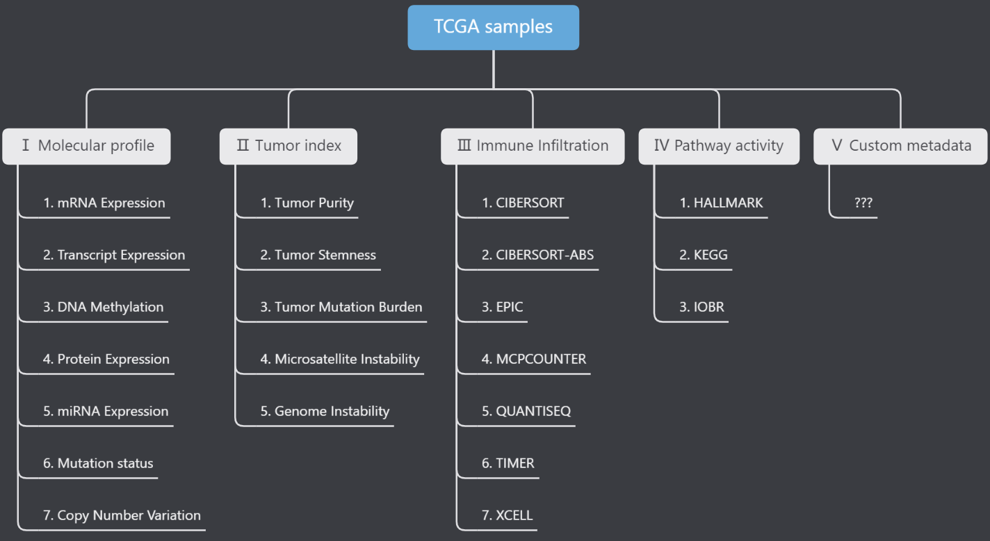
- “22 + X” data types: 4 main data type (Level1) including 22 minor types (Level2) are ensembled. In addition, users can upload customized TCGA sample metadata.
- Personalized operation: Several modules are provided for personalized analysis, like sample filtering/grouping, dataset modification.
2. Basic use
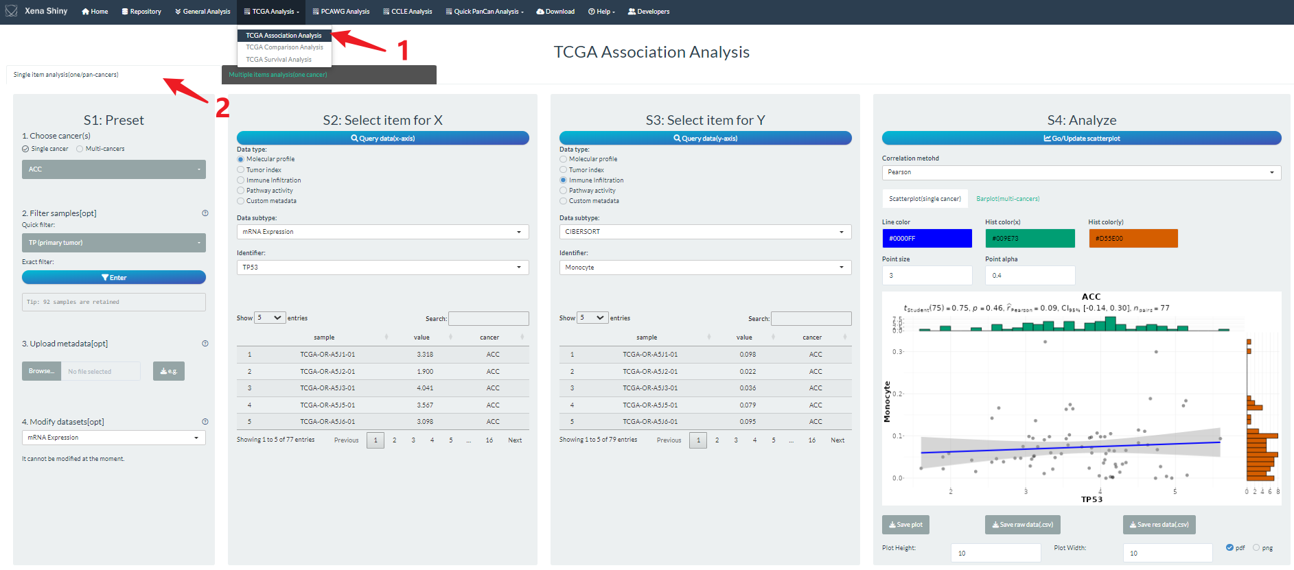
Take correlation analysis for example, we will introduce the basic pipeline.
(1) Firstly, once you enter the shiny app, click the TCGA Analysis navigation and select the “TCGA Association analysis” module.
(2) Then, select one panel for the corresponding mode. By default, you will be in the left panel which support one data analysis.
(3) Next, what you need do is to just follow the sequential steps from left to right.
- In step S1, you should choose the intended cancer type(s). In addition, we support some optional and personalized operations which will be introduced in other section below.
- In step S2 and S3, you need to assign the specific data. For correlation analysis, it involves X and Y variable selections of two items. For other analysis, you should also set the groups.
- In step S4, you can finally execute the correlation analysis and visualization. Some parameters can be modified like correlation method, point color. Notably, we support the result download for the table of raw or analyzed data, and figure of visualization.
3. Sample selection
Once you choose the cancer types(s), all the samples under the related project(s) will be chosen, such as tumor and normal samples. However, we need some filtering operations for specific analysis tasks.
For example, we only want the tumor samples for survival analysis or one gene-pair correlation under TP53 mutant samples.
In the 2nd part of S1 step , we provide the UI including two filters to select interesting subset of all samples.
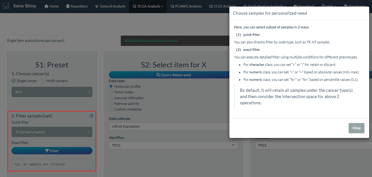
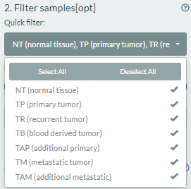
Firstly, users can directly perform the quick filter according to the tissue code types under the cancer(s) selections.
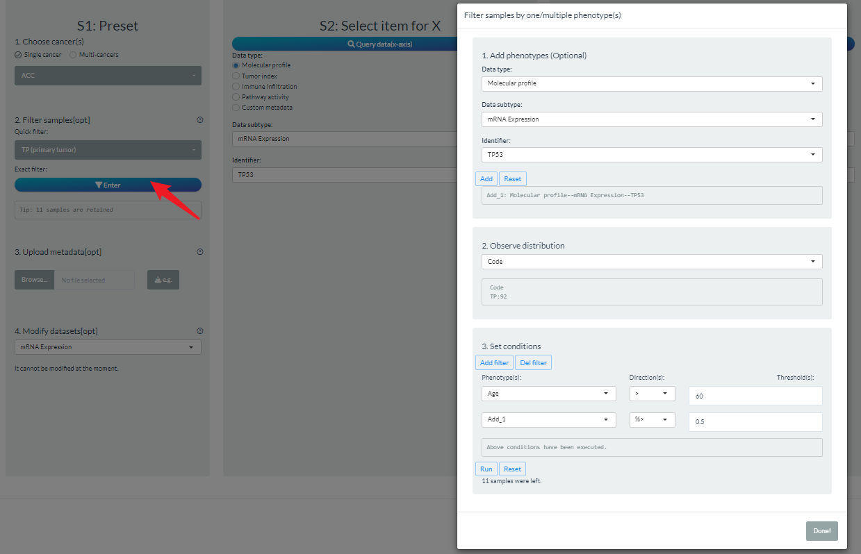
Secondly, users can perform the exact filter when entering the following example dialog box.
- By default, we have prepared several clinical phenotypes such as code, gender, age, stage. User can add any data as the extra filter conditions.
- According to the condition class, there are different filter operations.
- For character class, users can retain or discard some categories;
- For numeric class, users can set the cutoff based on absolute or percentile values.
- When setting multiple condition filters, each is executed independently and take the overall intersection finally.
Note: If you perform both quick and exact filters, the shared samples will be selected.
4. Custom metadata
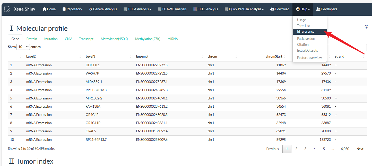
As the first figure above shown, we ensemble the TCGA feature data into 3 levels. Level1 and Level2 refer to the main and minor data types. Level3 refer to the specific item id. We have prepared 4 Level1 types which could be queried in detail from the Help→Id reference page.
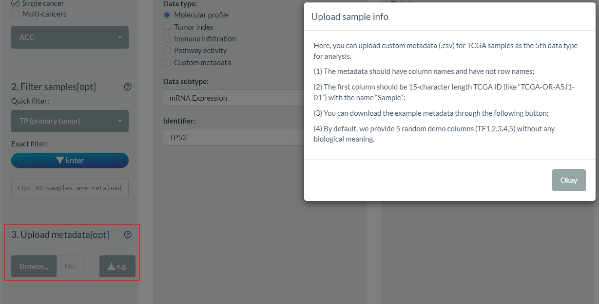
In addition, we allow users to upload customized TCGA metadata or annotation as the 5th Level1 type in the 3rd part of S1 step.
For the file to upload, it should be CSV format. Its first column must be standard TCGA sample id (TCGA-XX-XXXX-XX) with the column name “Sample”. As it is not necessary to include all TCGA samples, you can upload limited samples information according to your analysis task.
5. Modify datasets
Among the UCSC Xena data portal, there are great alternative datasets for the sample data type, like different normalization of mRNA expression, different array of DNA methylation. By default, we have set one common dataset for each Level2 data type (). Now, it is accessible for users to change the default dataset selection in the 4th part of S1 step.
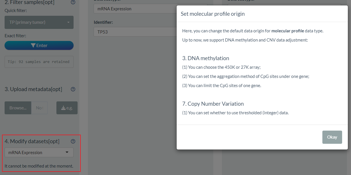
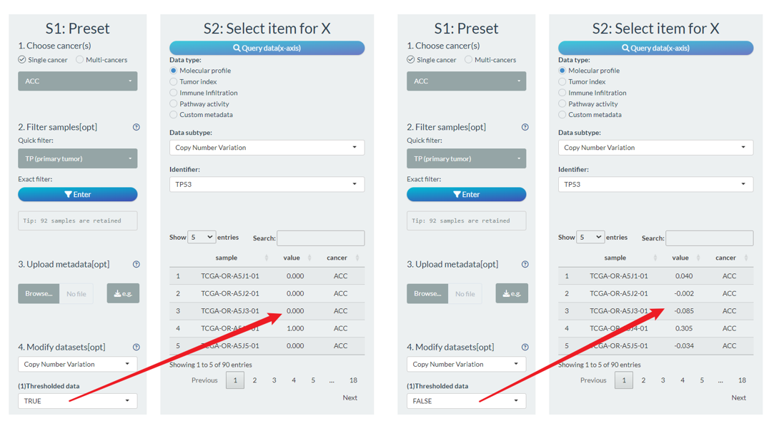
As the preliminary try, we temporarily allow the selection of DNA methylation and CNV data.
- For the CNV data, uses can set whether to use the threshold data (default is TRUE);
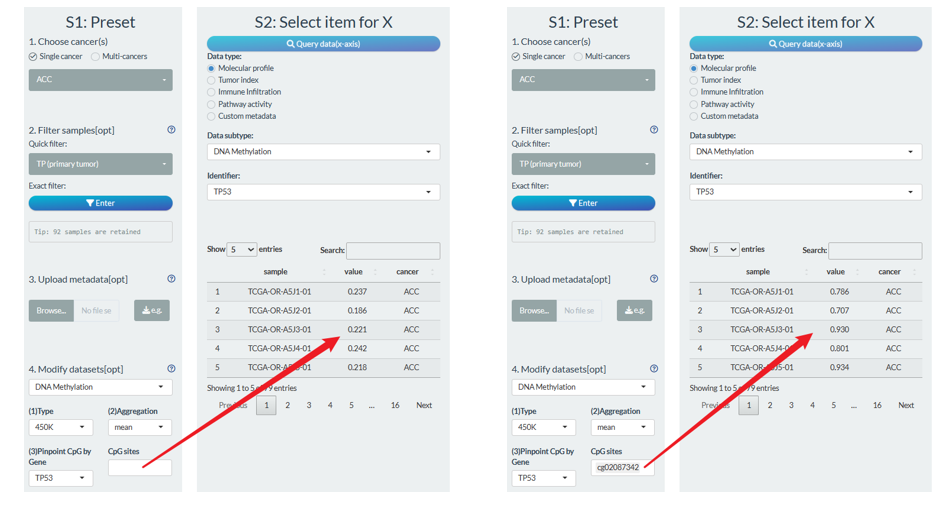
- For the DNA methylation, users can have more options. On the one hand, you can choose 450K or 27K array (only limited samples for 27K). As one gene often covers multiple CpG sites, the mean value will be calculated by default. You can change the aggregation methods and CpG range. For example, you can just consider one CpG site for one gene as follows (right figure).
Tip: The CpG Chromosomal coordinate information can be queried from Help→Id reference page.
In the future update, we will consider more options for other molecular profile data type, like mRNA expression.
6. Binary grouping
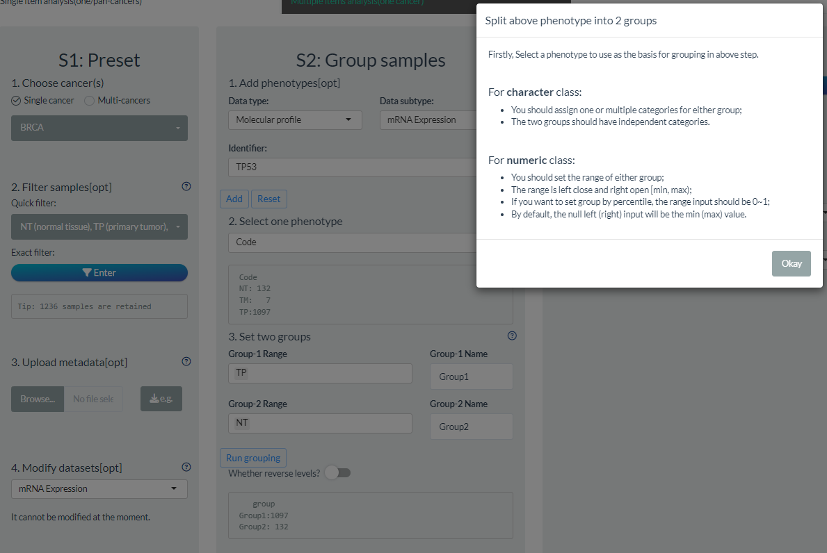
For comparison or survival analysis, it is necessary to divide samples into groups. Therefore, we design the module for binary grouping operation.
Take comparison analysis for example, you should firstly confirm the S1 preset. Like sample filtering, we preliminarily provide common clinical phenotypes and you can also add any data from ensembled features. However, only one could be considered as grouping condition.
- For character class, you can assign one or several categories for either group;
- For numeric class, you can set the min and max range of each group. Absolute and percentile value are all supported.
Please note it will cause a warning when existing shared samples between groups which should be avoided.
In addition, you can also set the group names and levels. By default, they are “Group1” and “Goup2” in order.
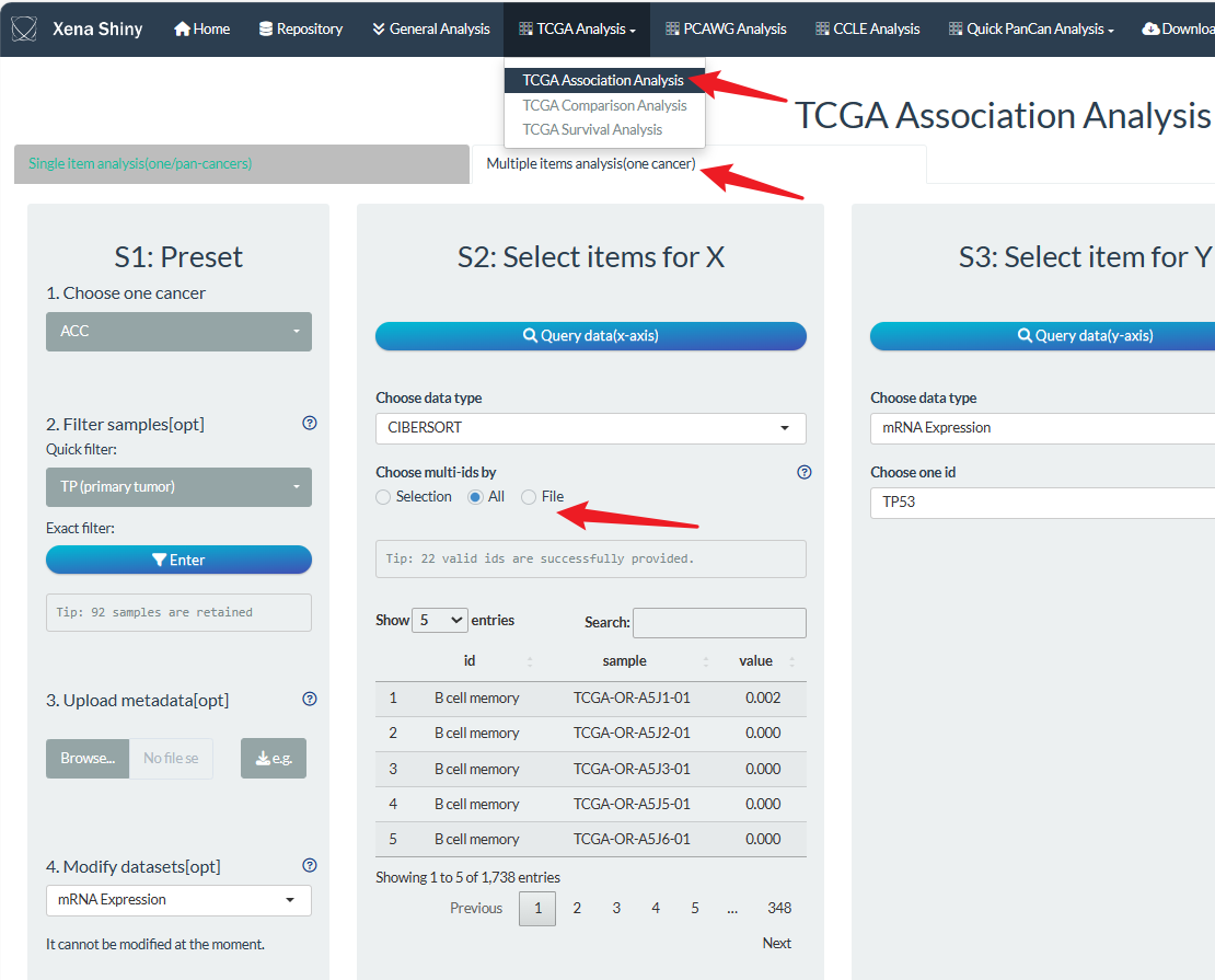
7. Multiple items selection
For the mode of multiple data on one cancer which is located in the second right panel of analysis page, users can perform batch analysis easily to screen significant items.
For example, we can find the most correlated immune infiltration with one gene expression. The main operation difference is involved the selection of multiple items.
Here, take batch correlation analysis for example, users can set multiple items in step S2 in three ways under one specific Level2 data type.
- Firstly, users can select some items one by one (left option “Selection”);
- Secondly, users can directly select all the ids (middle option “All”, like the figure below). However, it will take much time and cache to download molecular profile data. So, it will choose random 100 items for this Level1 type which need for better optimization in the future.
- Lastly, users can upload item file and see the format requirements by downloading the example file.