R-可视化--ggplot绘制散点图添加边际图

 1
 2
 3
 4
 5
 6
 7
 8
 9
10
11
12

data("mtcars")
df <- mtcars
df$name <- rownames(df)
df$cyl <- as.factor(df$cyl)
head(df[,c("name","cyl","mpg","wt")])
#                                name cyl  mpg    wt
# Mazda RX4                 Mazda RX4   6 21.0 2.620
# Mazda RX4 Wag         Mazda RX4 Wag   6 21.0 2.875
# Datsun 710               Datsun 710   4 22.8 2.320
# Hornet 4 Drive       Hornet 4 Drive   6 21.4 3.215
# Hornet Sportabout Hornet Sportabout   8 18.7 3.440
# Valiant                     Valiant   6 18.1 3.460

 1
 2
 3
 4
 5
 6
 7
 8
 9
10
11
12
13
14
15
16

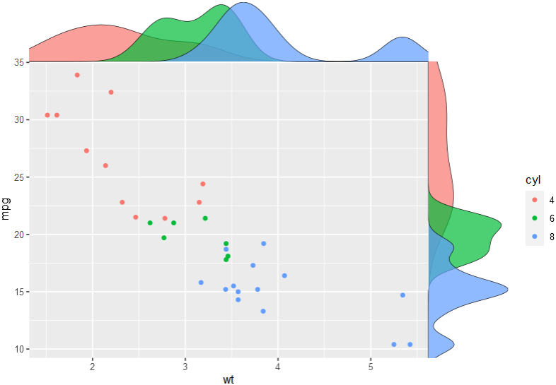
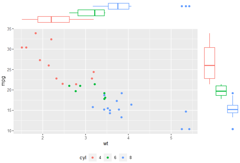
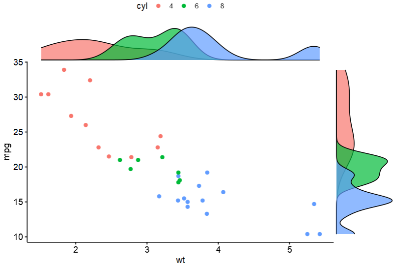
library(cowplot) 
p_main = ggplot(df, aes(x = wt, y = mpg, color = cyl))+
  geom_point()

p_right = axis_canvas(p_main, axis = "x")+
  geom_density(data = df, aes(x = wt, fill = cyl),
              alpha = 0.7, size = 0.2)

p_top = axis_canvas(p_main, axis = "y", coord_flip = TRUE)+
  geom_density(data = df, aes(x = mpg, fill = cyl),
                alpha = 0.7, size = 0.2)+
  coord_flip()

p1 = insert_xaxis_grob(p_main, p_right, grid::unit(.2, "null"), position = "top")
p2 =  insert_yaxis_grob(p1, p_top, grid::unit(.2, "null"), position = "right")
ggdraw(p2)

 1
 2
 3
 4
 5
 6
 7
 8
 9
10
11
12
13
14
15
16
17
18
19
20

library(patchwork)

p_main = ggplot(df, aes(x = wt, y = mpg, color = cyl)) + 
	geom_point() +
	theme(legend.position="bottom")
  
p_top = ggplot(df, aes(x = wt, color = cyl)) + 
	geom_boxplot() + theme_void() +
	theme(legend.position = "none")


p_right = ggplot(df, aes(x = mpg, color = cyl)) + 
	geom_boxplot() + theme_void() +
	theme(legend.position = "none") +
	coord_flip()

p = p_top + plot_spacer() + p_main + p_right +
    plot_layout(ncol = 2, nrow = 2, 
    			heights = c(1, 5),  
    			widths = c(5, 1))

1
2
3
4
5
6
7

library(ggpubr)
ggscatterhist(
	df, x = "wt", y = "mpg",
	color = "cyl",
	margin.plot = "density",  # ("density", "histogram", "boxplot"),
	margin.params = list(color = "black",fill="cyl")
)