桑基图(sankey plot)是一种特定类型的流图,用于描述一组值到另一组值的流向;理论上来表示前一组值与后一组值存在一定的逻辑关系。从泛化角度来看,也可用于呈现多组间的构成比例关系。从这个角度来看,冲积图(alluvial plot)就是一种特殊的桑基图。
- ggsankey包的官方教程:https://github.com/davidsjoberg/ggsankey
1
2
# install.packages("devtools") devtools::install_github("davidsjoberg/")
1、构图要素
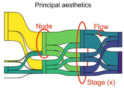
(1)图形组成
- 一整列对应的每一组值表示一个stage,每个stage由若干个node组成;
- 相邻两个stage的node之间可存在流向关系,称为flow。
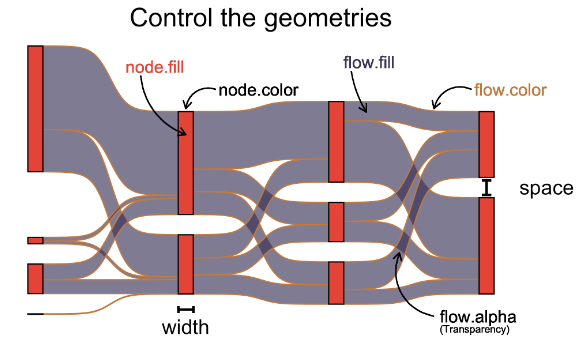
(2)图形参数
fill设置填充颜色,可进一步分为node.fill与flow.fill;color设置边框颜色,可进一步分为node.color与flow.color;width设置node的宽度,flow.alpha设置flow的不透明度,space设置同组内node的间距。
2、准备数据
|
|
- 汽车型号数据mtcars
|
|
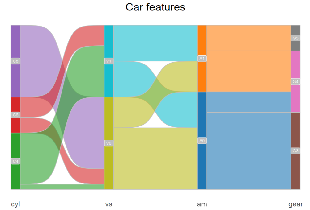
3、绘制桑基图
主要函数
geom_sankey()绘制桑基图,主要参数见1.2geom_sankey_text()/geom_sankey_label()添加node标签,相关参数同geom_text/label
|
|
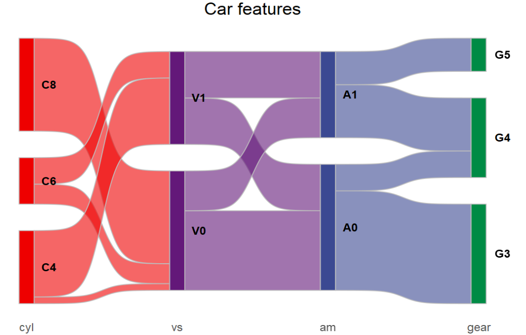
4、绘制冲击图
Alluvial plots are very similiar to sankey plots but have no spaces between nodes and start at y = 0 instead being centered around the x-axis.
主要函数:
geom_alluvial()绘制冲积图,主要参数同geom_sankey()geom_alluvial_text()/geom_alluvial_label()添加node标签,相关参数同geom_text/label
|
|