一、ggplot绘制基础箱图
0、示例数据
|
|
1、基础绘图
|
|
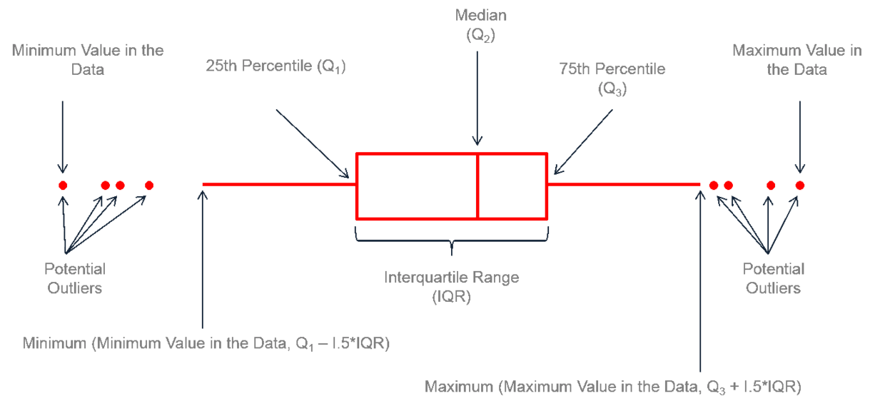
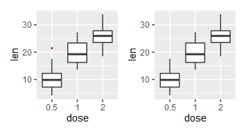
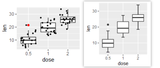
2、离群点相关
|
|
3、添加随机抖动点/whisker须线
|
|
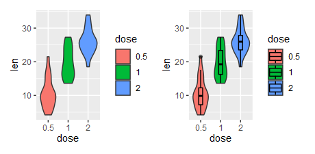
4、嵌套小提琴图
|
|
二、ggpubr进行两/多组比较
ggpubr包提供了组间比较的分析函数与可视化函数,主要参考自http://www.sthda.com/english/articles/24-ggpubr-publication-ready-plots/76-add-p-values-and-significance-levels-to-ggplots/
0、示例数据
|
|
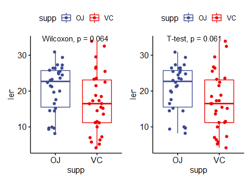
1、组间差异检验
1.1 两组间比较
(1)选择有参法还是无参法;(2)能否进行配对比较
|
|
1.2 多分组比较
|
|
2、绘制箱图
2.1 两组间比较
(1)不同比较方式
|
|
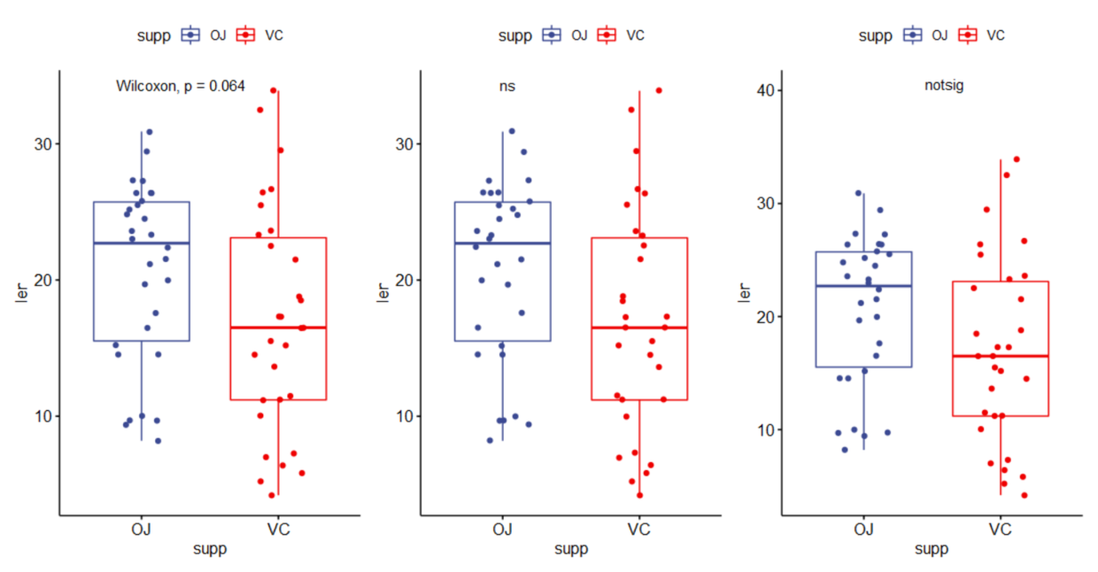
(2)标签显示格式
|
|
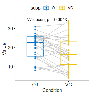
(3)配对分析
|
|
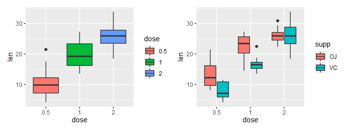
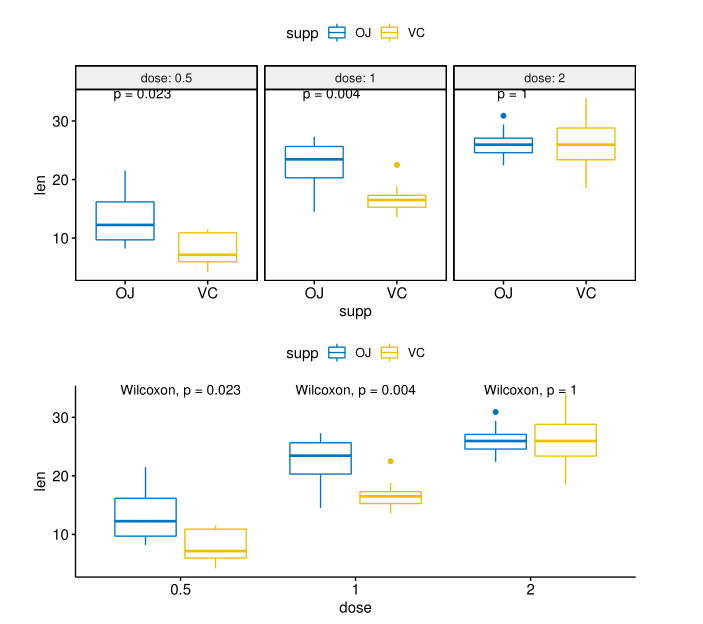
(4)考虑其它分组变量
|
|
2.2 多组间比较
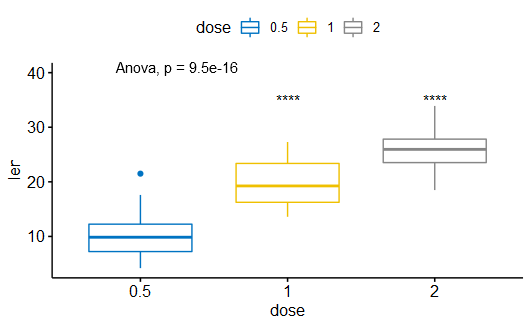
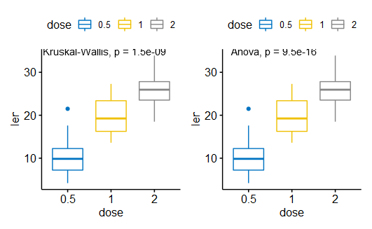
(1)方差分析
|
|
(2)两两比较
|
|
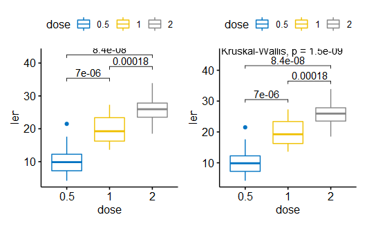
|
|