使用igraph包进行网络结构分析与可视化

1、创建与查看igraph对象

1.1 示例数据

igraph包提供了很多创建igraph对象的函数与思路。这里采用常用的基于data.frame的格式创建。
示例数据来自STRINGdb的PPI蛋白互作数据以及对应基因的上下调信息

 1
 2
 3
 4
 5
 6
 7
 8
 9
10
11
12
13
14
15
16
17
18
19
20
21
22
23
24
25
26
27
28
29
30
31
32
33
34
35
36
37
38
39
40
41
42
43
44
45


library(STRINGdb)
library(tidyverse)
string_db <- STRINGdb$new(version="11", 
                          species=9606,
                          score_threshold=200, 
                          input_directory="")
data(diff_exp_example1)
genes = rbind(head(diff_exp_example1,30),
              tail(diff_exp_example1,30))
head(genes)
genes_mapped <- string_db$map(genes, "gene" )
head(genes_mapped)
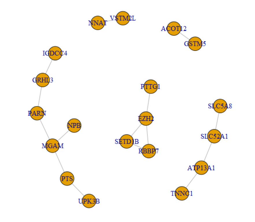
ppi = string_db$get_interactions(genes_mapped$STRING_id) %>% distinct()
edges = ppi %>% 
  dplyr::left_join(genes_mapped[,c(1,4)], by=c('from'='STRING_id')) %>% 
  dplyr::rename(Gene1=gene) %>% 
  dplyr::left_join(genes_mapped[,c(1,4)], by=c('to'='STRING_id')) %>% 
  dplyr::rename(Gene2=gene) %>% 
  dplyr::select(Gene1, Gene2, combined_score)

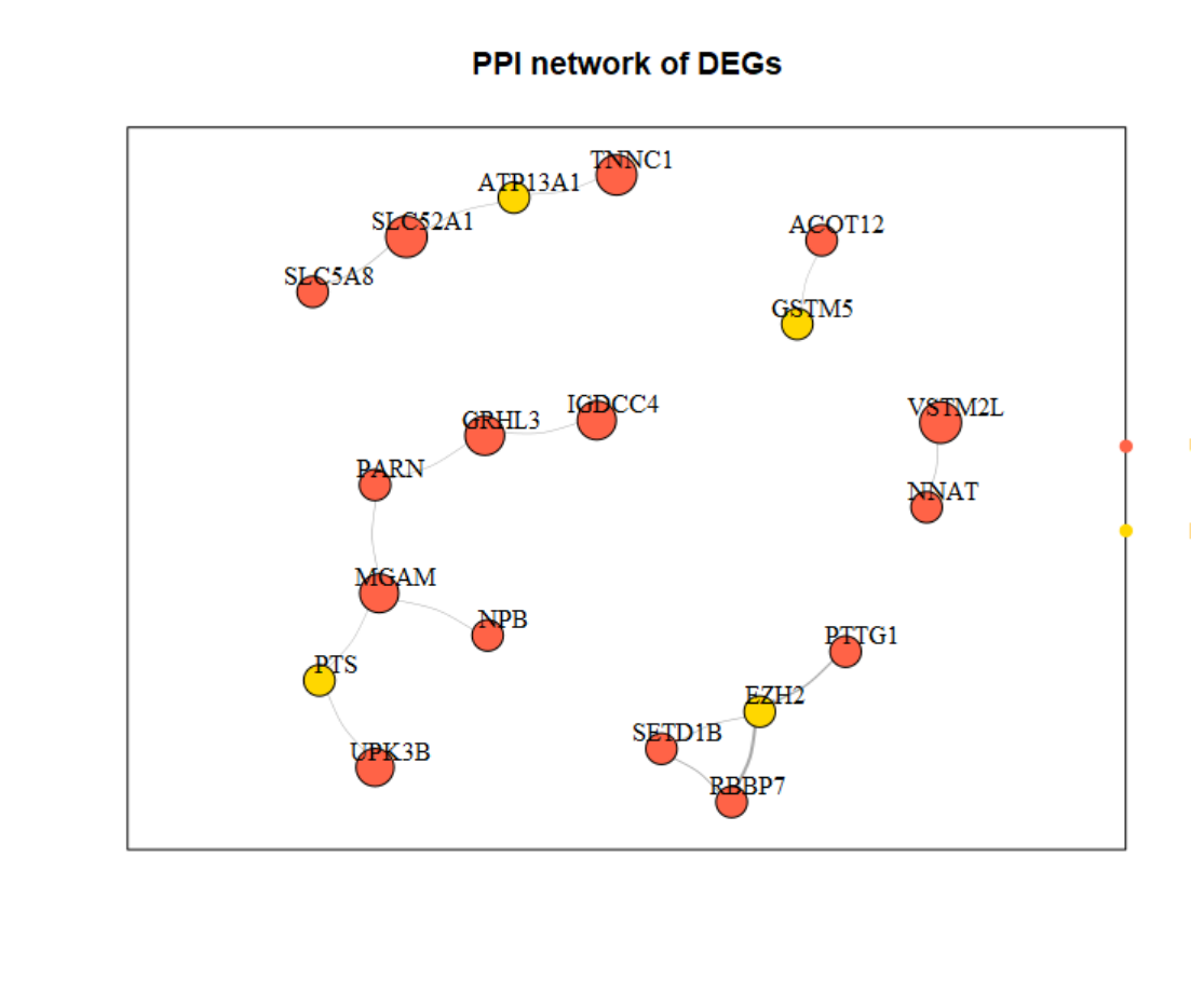
nodes = genes_mapped %>% 
  dplyr::filter(gene %in% c(edges$Gene1, edges$Gene2)) %>% 
  dplyr::mutate(log10P = -log10(pvalue),
                direction = ifelse(logFC>0,"Up","Down")) %>% 
  dplyr::select(gene, log10P, logFC, direction)

###边信息
head(edges)
#   Gene1   Gene2 combined_score
# 1 UPK3B     PTS            244
# 2 GSTM5  ACOT12            204
# 3 GRHL3  IGDCC4            238
# 4 TNNC1 ATP13A1            222
# 5  NNAT  VSTM2L            281
# 6  EZH2   RBBP7            996

###节点信息
head(nodes)
#      gene   log10P    logFC direction
# 1  VSTM2L 3.992252 3.333461        Up
# 2   TNNC1 3.534468 2.932060        Up
# 3    MGAM 3.515558 2.369738        Up
# 4  IGDCC4 3.290137 2.409806        Up
# 5   UPK3B 3.248490 2.073072        Up
# 6 SLC52A1 3.227019 3.214998        Up

1.2 创建对象

使用graph_from_data_frame()函数创建

 1
 2
 3
 4
 5
 6
 7
 8
 9
10
11
12
13


library(igraph)
library(tidyverse)
g1 = graph_from_data_frame(d = edges, #交代边信息
                           vertices = nodes, #交代点信息
                           directed = FALSE)
g1
# IGRAPH 3eb2403 UN-- 19 15 -- 
# + attr: name (v/c), log10P (v/n), logFC (v/n), direction (v/c), combined_score
# | (e/n)
# + edges from 3eb2403 (vertex names):
#  [1] UPK3B  --PTS     GSTM5  --ACOT12  IGDCC4 --GRHL3   TNNC1  --ATP13A1 VSTM2L --NNAT   
#  [6] EZH2   --RBBP7   PTTG1  --EZH2    GRHL3  --PARN    SLC52A1--ATP13A1 SETD1B --EZH2   
# [11] SETD1B --RBBP7   SLC52A1--SLC5A8  MGAM   --PTS     MGAM   --NPB     MGAM   --PARN   

第一行的UN--的4个占位符：（1）D/U, 表示是否为有向图；（2）N，表示节点node是否有name属性；（3）W，表示边edge是否有weight属性；（4）B，表示节点node是否有type属性。

后面紧接着的两个数字（19 15）分别表示节点总数与边总数

第二行则表示点v/边e/图g目前由哪些属性；后面的第二个字母则表示属性字符类型：n:numeric; c:character;l:logical

1.3 查看对象

基本统计

 1
 2
 3
 4
 5
 6
 7
 8
 9
10
11
12
13
14
15
16
17
18
19
20
21
22


###(1)边信息
E(g1)
# + 15/15 edges from 3eb2403 (vertex names):
# [1] UPK3B  --PTS     GSTM5  --ACOT12  IGDCC4 --GRHL3   TNNC1  --ATP13A1 VSTM2L --NNAT 
# ...

as_ids(E(g1)) %>% str()
# chr [1:15] "UPK3B|PTS" "GSTM5|ACOT12" "IGDCC4|GRHL3" "TNNC1|ATP13A1" ...
###多少条边
ecount(g1)
# [1] 15

###(2)节点信息
V(g1)
# + 19/19 vertices, named, from 3eb2403:
# [1] VSTM2L  TNNC1   MGAM    IGDCC4  UPK3B   SLC52A1 GRHL3   SLC5A8  GSTM5   NNAT 

as_ids(V(g1)) %>% str()
# chr [1:19] "VSTM2L" "TNNC1" "MGAM" "IGDCC4" "UPK3B" "SLC52A1" "GRHL3" ...
###多少个点
vcount(g1)
# [1] 19

节点的邻居

 1
 2
 3
 4
 5
 6
 7
 8
 9
10
11
12
13


###节点邻居（下面三个命令结果一样）
V(g1)[nei("GRHL3")]
neighbors(g1,"GRHL3")
g1[["GRHL3"]]

##包含节点的有哪些
g1[["GRHL3",edges=TRUE]]


###针对有向图
g1[["GRHL3",]] #以GRHL3为起始点的邻居节点
g1[[,"GRHL3"]] #以GRHL3为终点的邻居节点
g1[["GRHL3",,edges=TRUE]] #以GRHL3为起始点的边

节点之间的距离

1
2
3
4
5
6
7


##计算两节点之间的距离
##如果存在边权重，可计算权重距离和
##如果两个节点没有公共节点，则计算距离为0
distances(g1, v=c("PTS","NPB"), to=c("IGDCC4","UPK3B","NPB"))
#     IGDCC4 UPK3B NPB
# PTS      4     1   2
# NPB      4     3   0

1.4 igraph对象转为data.frame

1
2
3
4
5
6
7
8
9


#单独保存边信息
as_data_frame(g1, what = "edges") %>% head()

#单独保存点信息
as_data_frame(g1, what = "vertices") %>% head()

#同时保存点和边的信息
as_data_frame(g1, what = "both") %>% head()
#为包含两个表格的list对象

2、edge与vertex属性

2.1 edge边属性

 1
 2
 3
 4
 5
 6
 7
 8
 9
10
11
12
13
14
15


edge_attr(g1) %>% names() 
# edge_attr_names(g1)
#[1] "combined_score"

edge_attr(g1)$combined_score
# E(g1)$combined_score
# [1] 244 204 238 222 281 996 598 225 226 291 415 294 210 237 266

#增加边属性
edge_attr(g1)$weight = edge_attr(g1)$combined_score
edge_attr(g1)$type = ifelse(edge_attr(g1)$combined_score>500, "strong","weak")
#删除边属性
g1 <- delete_edge_attr(g1, "type")
edge_attr(g1) %>% names()
# [1] "combined_score" "weight"

2.2 vertex点属性

1
2
3
4
5
6
7


vertex_attr(g1) %>% names()
#[1] "name"      "log10P"    "logFC"     "direction"

vertex_attr(g1)$name
#V(g1)$name
# [1] "VSTM2L"  "TNNC1"   "MGAM"    "IGDCC4"  "UPK3B"   "SLC52A1" "GRHL3"   "SLC5A8" 
# ...

2.3 graph图属性

1
2
3
4


g1 <- set_graph_attr(g1, "name", "PPI network")
graph_attr(g1)
# $name
# [1] "PPI network"

2.4 增删点与边

增加点

1
2
3
4
5
6
7
8
9



vertex_attr(g1) %>% names()
# [1] "name"      "log10P"    "logFC"     "direction"
#增加两个节点
g1 %>% add_vertices(nv = 2,
                    attr = list(name=c("TP53","APC"),
                                log10P=c(3,2),
                                logFC=c(2,1),
                                direction=c("Up","Down")))

增加边

1
2
3
4
5
6


edge_attr(g1) %>% names()
# [1] "combined_score" "weight" 
#增加两条边
g1 %>% add_edges(c("PTTG1","NPB","ACOT12","SLC5A8"),
                 attr = list(combined_score = c(500,500),
                             weight = c(300,300)))

删除点

1
2
3


V(g1)
g1 %>%  delete_vertices(, c(1,5)) %>% #根据序号下标
  delete_vertices("GSTM5") #直接根据名字

删除边

1
2
3


E(g1)
g1 %>% delete_edges(1) %>% #根据序号下标
  delete_edges("NPB|MGAM") #直接边的节点组成

3、节点重要性网络分析

3.1 点度中心性degree

与目标节点直接相连的节点数

 1
 2
 3
 4
 5
 6
 7
 8
 9
10
11
12
13
14
15
16


# mode参数主要考虑有向图的可能
degree(g1, mode="all")
# VSTM2L   TNNC1    MGAM  IGDCC4   UPK3B SLC52A1   GRHL3  SLC5A8   GSTM5    NNAT   PTTG1 
#     1       1       3       1       1       2       2       1       1       1       1 
# ATP13A1  ACOT12  SETD1B     NPB    EZH2    PARN     PTS   RBBP7 
#     2       1       2       1       3       2       2       2 

# normalized = T表示相对点度中心性
# 即divided by n-1, where n is the number of vertices in the graph.
degree(g1, mode="all", normalized = T)
# VSTM2L      TNNC1       MGAM     IGDCC4      UPK3B    SLC52A1      GRHL3     SLC5A8 
# 0.05555556 0.05555556 0.16666667 0.05555556 0.05555556 0.11111111 0.11111111 0.05555556 
# GSTM5       NNAT      PTTG1    ATP13A1     ACOT12     SETD1B        NPB       EZH2 
# 0.05555556 0.05555556 0.05555556 0.11111111 0.05555556 0.11111111 0.05555556 0.16666667 
# PARN        PTS      RBBP7 
# 0.11111111 0.11111111 0.11111111

3.2 紧密度中间性closeness

目标节点到其余所有节点的最短（权重）距离均值的倒数

 1
 2
 3
 4
 5
 6
 7
 8
 9
10
11
12
13
14


closeness(g1, mode="all", weights=NA)
# 参数weights表示计算最短距离时是否考虑边的权重
# VSTM2L       TNNC1        MGAM      IGDCC4       UPK3B     SLC52A1       GRHL3 
# 0.003086420 0.003436426 0.004201681 0.004048583 0.004065041 0.003460208 0.004132231 
# SLC5A8       GSTM5        NNAT       PTTG1     ATP13A1      ACOT12      SETD1B 
# 0.003436426 0.003086420 0.003086420 0.003448276 0.003460208 0.003086420 0.003460208 
# NPB        EZH2        PARN         PTS       RBBP7 
# 0.004115226 0.003472222 0.004184100 0.004149378 0.003460208

# Warning message:
# In closeness(g1, mode = "all", weights = NA) :
#   At centrality.c:2874 :closeness centrality is not well-defined for disconnected graphs

#同样可设置normalized参数是否进行标准化

由于提供的PPI网络存在断连的情况，所以会出现上面的warning

3.3 介数中间性betweenness

除目标节点外所有节点间的最短(权重)距离是否经过目标节点（的次数）

1
2
3
4
5
6
7


betweenness(g1, directed = FALSE, weights=NA)
# VSTM2L   TNNC1    MGAM  IGDCC4   UPK3B SLC52A1   GRHL3  SLC5A8   GSTM5    NNAT   PTTG1 
# 0       0      11       0       0       2       5       0       0       0       0 
# ATP13A1  ACOT12  SETD1B     NPB    EZH2    PARN     PTS   RBBP7 
# 2       0       0       0       2       8       5       0 

#同样可设置normalized参数是否进行标准化

4、网络可视化

1

plot(g1)

图形的调整参数涉及如下三个方面

（1）节点与节点的标签；

Introduction from [Kateto tutorial](https://kateto.net/networks-r-igraph)

（2）边

（3）其它

例如，设置节点的颜色与差异基因上下调相关，节点大小与上下调程度相关，边的宽度与蛋白互作程度相关

 1
 2
 3
 4
 5
 6
 7
 8
 9
10
11
12
13
14
15
16
17
18
19
20
21
22
23
24
25
26
27


#设置节点颜色--上下调方向
vcol=vertex_attr(g1)$direction
vcol[vcol=="Up"]="tomato"
vcol[vcol=="Down"]="gold"
V(g1)$color=vcol

# 设置节点大小--上下调程度
vsize=vertex_attr(g1)$logFC %>% abs() %>% round(1)
V(g1)$size=vsize+10


# 设置线的宽度(相对值)
E(g1)$width=edge_attr(g1)$combined_score/500

set.seed(123)
plot(g1, 
     vertex.label.color="black", 
     vertex.label.cex=1, 
     vertex.label.dist=1, 
     edge.curved=0.2,
     layout=layout_with_fr,
     #layout=layout.auto(g1),
     frame = TRUE, main="PPI network of DEGs")
legend("right", legend = c("Up","Down"), pch=21,
       col=c("tomato","gold"), 
       pt.bg=c("tomato","gold"), 
       pt.cex=1, cex=.8, bty="n", ncol=1)

关于layout参数，layout.auto()函数可根据网络组成，选择较为合适的布局：（1）connected and vcount<=100: kk；（2）vcount<=1000:fr；（3）else: drl

Layouts from [Kateto tutorial](https://kateto.net/networks-r-igraph)

ggraph包建立在ggplot2绘图框架上，可用于可视化igraph对象，具体用法以后有机会再学。

1、创建与查看igraph对象#

1.1 示例数据#

1.2 创建对象#

1.3 查看对象#

1.4 igraph对象转为data.frame#

2、edge与vertex属性#

2.1 edge边属性#

2.2 vertex点属性#

2.3 graph图属性#

2.4 增删点与边#

3、节点重要性网络分析#

3.1 点度中心性degree#

3.2 紧密度中间性closeness#

3.3 介数中间性betweenness#

4、网络可视化#