1、关于GAM非线性回归

(1) n阶多项式

  • 如前所说,线性回归的假设是每个预测变量与输出变量之间为线性相关。即类似 y = ax + b

  • 当预测变量与输出变量之间为非线性相关,即呈曲线特征时,可尝试使用高阶多项式进行拟合。 $$ y = \beta_0 + \beta_1x + \beta_2x^2 + …+\beta_nx^n + \varepsilon $$ 正交多项式介绍及应用- 优化与算法- 博客园

  • 一般拟合高阶多项式时,除了最高阶n外,还会包括所有低阶项(1,2,3… n-1)次幂。目的是为了避免最值点必须处于x=0的位置。

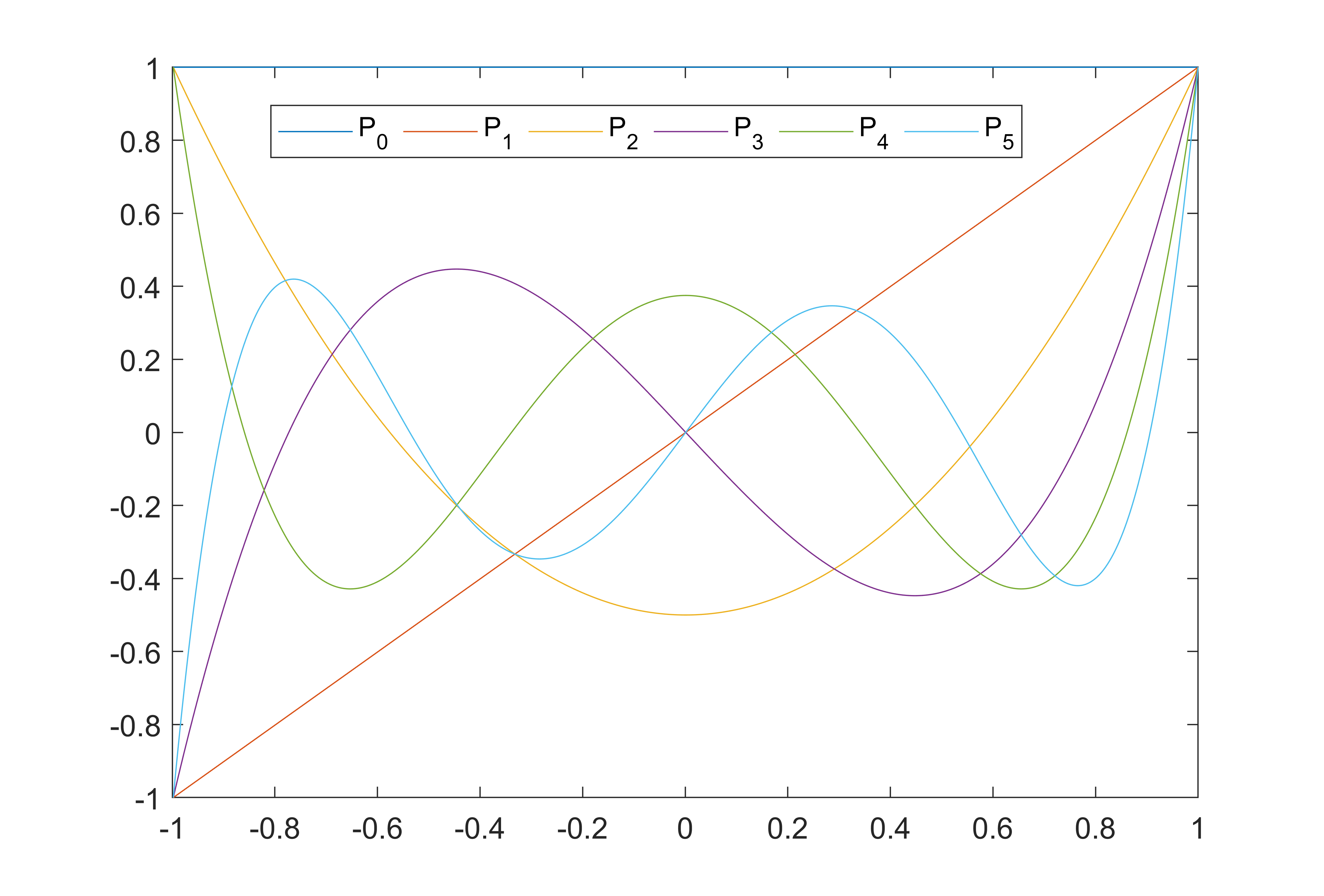
  • 样条曲线是分段的多项式函数:将预测变量分为若干区域,每个区域单独拟合一个多项式曲线。相邻的多项式之间的连接成为knot。

(2) GAM

  • GAM会尝试将每个预测变量与输出变量关系拟合为平滑曲线,通常是多个样条曲线的组合,其中每一个样条曲线称为基函数。

    • 对于预测变量Xi,平滑函数可以表示为如下。a表示每个基函数的权重。

    $$ f(x_i) = a_1b_1(x_i)+a_2b_2(x_i)+…+a_nb_n(x_n) $$

  • 所以GAM广义加性模型公式表示为: $$ y = \beta_0 + f_1(x_1) + f_2(x_2) + … + f_n(x_n) + \varepsilon $$

上一节提到的通用线性模型公式为: $$ y = \beta_0 + \beta_1x_1 + \beta_2x_2 + … + \beta_nx_n + \varepsilon $$ 可以这么理解:通用线性模型是广义加性模型的特例。

2、mlr建模

训练数据与目的同上一节

1
2
library(mlr3verse)
library(tidyverse)

2.1 臭氧水平空气质量数据

 1
 2
 3
 4
 5
 6
 7
 8
 9
10
11
12
13
14
15
16
17
18
19
20
21
22
23
24
data(Ozone, package = "mlbench")
colnames(Ozone) = c("Month", "Date", "Day", "Ozone", "Press_height",
                    "Wind", "Humid", "Temp_Sand", "Temp_Monte", 
                    "Inv_height", "Press_grad", "Inv_temp", "Visib")
Ozone2 = Ozone %>% 
  dplyr::mutate(across(where(is.factor), as.numeric)) %>% 
  na.omit()
str(Ozone2)
# 'data.frame':	203 obs. of  13 variables:
#  $ Month       : num  1 1 1 1 1 1 1 1 1 1 ...
#  $ Date        : num  5 6 7 8 9 12 13 14 15 16 ...
#  $ Day         : num  1 2 3 4 5 1 2 3 4 5 ...
#  $ Ozone       : num  5 6 4 4 6 6 5 4 4 7 ...
#  $ Press_height: num  5760 5720 5790 5790 5700 5720 5760 5780 5830 5870 ...
#  $ Wind        : num  3 4 6 3 3 3 6 6 3 2 ...
#  $ Humid       : num  51 69 19 25 73 44 33 19 19 19 ...
#  $ Temp_Sand   : num  54 35 45 55 41 51 51 54 58 61 ...
#  $ Temp_Monte  : num  45.3 49.6 46.4 52.7 48 ...
#  $ Inv_height  : num  1450 1568 2631 554 2083 ...
#  $ Press_grad  : num  25 15 -33 -28 23 9 -44 -44 -53 -67 ...
#  $ Inv_temp    : num  57 53.8 54.1 64.8 52.5 ...
#  $ Visib       : num  60 60 100 250 120 150 40 200 250 200 ...
#  - attr(*, "na.action")= 'omit' Named int [1:163] 1 2 3 4 10 11 17 18 20 24 ...
#   ..- attr(*, "names")= chr [1:163] "1" "2" "3" "4" ...

2.2 确定预测目标与训练方法

1
2
3
4
5
##(1)确定预测目标:根据每天的空气相关记录数据,预测那一天的臭氧水平
task_regr = as_task_regr(Ozone2, target = "Ozone")

##(2)使用线性回归模型
learner = lrn("regr.gam")

2.3 特征筛选建模

参考上一节,有两种筛选思路。如下选取第二种筛选最佳组合的方式

 1
 2
 3
 4
 5
 6
 7
 8
 9
10
11
12
13
14
15
16
17
18
19
20
21
22
23
24
25
26
27
28
29
30
31
32
33
34
35
36
37
38
39
40
41
42
43
44
45
46
47
resampling = rsmp("cv")
resampling$param_set$values$folds = 3
measure = msr("regr.mse")
instance = FSelectInstanceSingleCrit$new(
  task = task_regr,
  learner = learner,
  resampling = resampling,
  measure = measure,
  terminator = trm("none")
)
instance

future::plan("multisession")
fselector = fs("sequential")
fselector$param_set$values
# <ParamSet>
#              id    class lower upper nlevels        default value
# 1: min_features ParamInt     1   Inf     Inf              1     1
# 2: max_features ParamInt     1   Inf     Inf <NoDefault[3]>      
# 3:     strategy ParamFct    NA    NA       2            sfs   sfs
fselector$optimize(instance)
# [1] "Humid"        "Inv_height"   "Inv_temp"     "Month"        "Press_height" "Temp_Monte"   "Temp_Sand"    "Visib"

instance$result_y
# regr.mse 
# 18.55917

task_regr$select(instance$result_feature_set)
learner$train(task_regr)
learner$model
# Family: gaussian 
# Link function: identity 

# Formula:
# Ozone ~ Humid + Inv_height + Inv_temp + Month + Press_height + 
#     Temp_Monte + Temp_Sand + Visib
# Total model degrees of freedom 9 

# GCV score: 19.72521 


##交叉验证
resampling = rsmp("cv")
rr = resample(task_regr, learner, resampling)
rr$aggregate(msrs(c("regr.mse")))
# regr.mse 
# 19.32496