机器学习基于R包mlr3(6)--分类--决策树与随机森林

1、决策树基础

1.1 决策树的构成

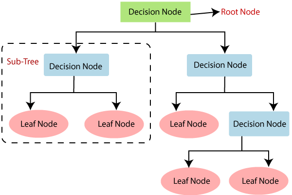
（1）决策树由节点组成，可分为决策节点(Decision tree)与叶节点(leaf node)。

（2）从上到下的第一个节点也称为根节点(Root Node)。根节点到叶节点的最长距离称为树的深度。

（3）对于每一个决策节点，选择样本集的一个最佳预测变量，确定最佳的阈值，进行二分类；最后根据叶节点类别的众数进行分类（均数进行回归）。

Machine Learning Decision Tree Classification Algorithm - Javatpoint

在决策树中有两个关键问题：

（1）如何选择最佳的预测变量？以及如何确定其阈值？

（2）如何防止决策树过拟合

1.2 基尼系数

（1）决策树为了使表示数据杂乱程度的不纯度减小，选择预测变量的最佳cut-off进行分割。当分割出来的每个组中的标签大部分属于同种标签时，不纯度会变小。

每一组的复杂度可通过基尼指数表示。其值越小，表示数据纯度越高
分割前后的数据复杂度变化可通过基尼增益表示。其值越大，表示数据的纯度变得越高。

（2）基尼指数与基尼增益的计算方法如下图所示：

如公式所示，对于二分类任务的基尼指数取值范围应为0~0.5之间。当等于0时，表示由同一种标签样本组成；当等于0.5时，表示两个标签样本各占一半。

微信图片_20220414092907

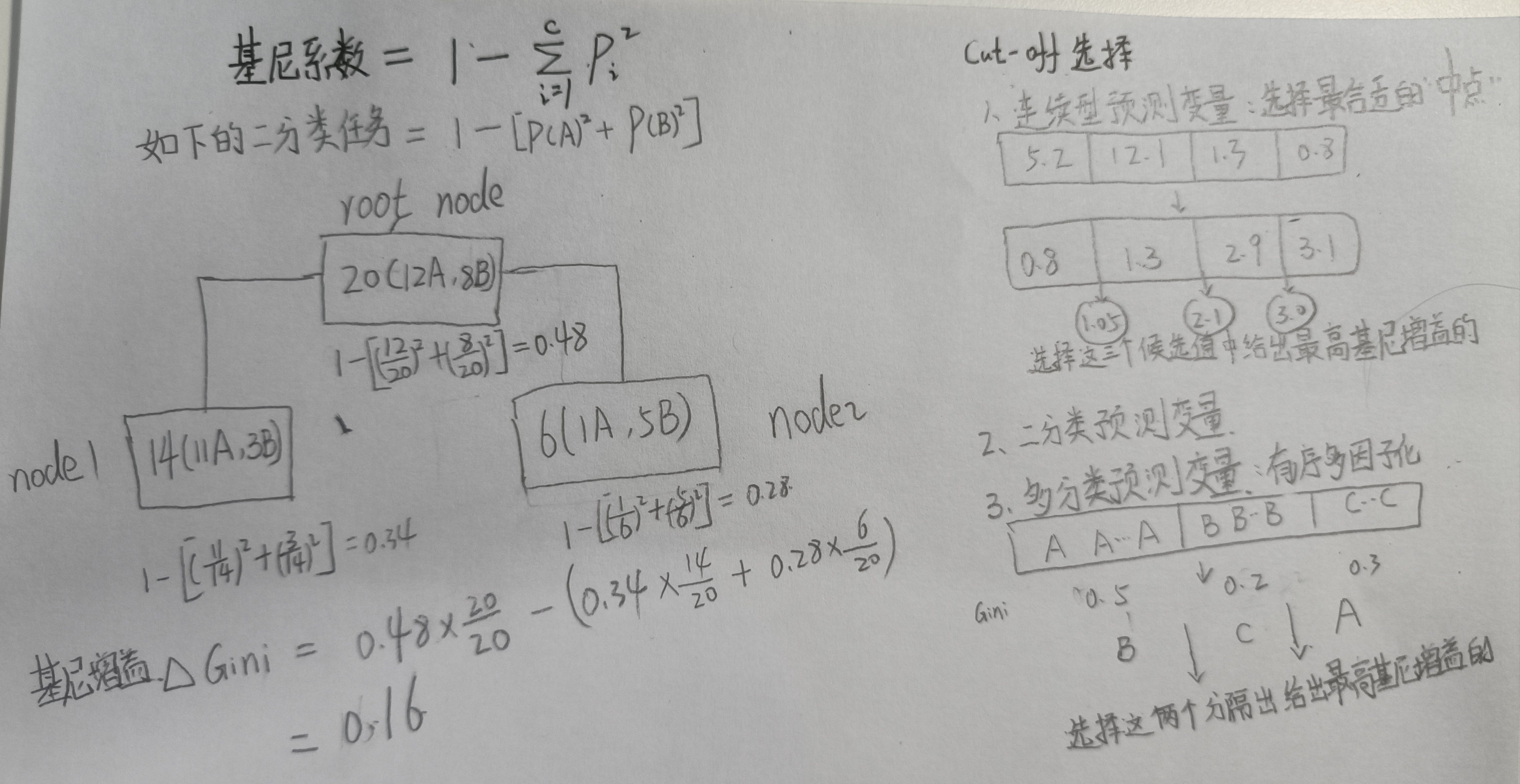
（3）比较不同预测变量的基尼增益，其实就是比较把不同预测变量的最佳分割cut-off下的基尼增益。

具体对于不同类型的预测变量，如上图所示，有不同的选择方法（从若干候选值中选择一个最佳的，作为该预测变量的代表）

1.3 防止决策树过拟合

如果不对决策树做出限制，它会一直划分节点，直至所有的叶节点都是只有一个类别的纯节点。这是决策树过拟合的主要原因。
防止过拟合的思路有两种–
- ① 先生成一颗冗长的树，再回过头修剪；
- ② 提前定义好规则，防止树出现过拟合。
关于第二种思路，有如下4个角度（超参数）

（1）直接限制最长深度；

（2）每一次划分所引起的最小性能改进（cp值，类似于基尼增益）；

（3）叶节点size：如果划分一个节点会导致叶节点中包含的样本数少于规定值，则不会划分；

（4）决策节点size：如果决策节点少于规定值，则不会被划分。（就被视为了叶节点）

2、决策树mlr建模

2.1 动物特征数据集

 1
 2
 3
 4
 5
 6
 7
 8
 9
10
11
12
13
14
15
16
17
18
19
20
21
22
23
24
25
26


data(Zoo, package = "mlbench")
#将逻辑变量(True/False)转为数值型因子变量
Zoo2 = Zoo %>% 
        dplyr::mutate(across(where(is.logical), as.factor))
str(Zoo2)
# 'data.frame':	101 obs. of  17 variables:
#  $ hair    : Factor w/ 2 levels "FALSE","TRUE": 2 2 1 2 2 2 2 1 1 2 ...
#  $ feathers: Factor w/ 2 levels "FALSE","TRUE": 1 1 1 1 1 1 1 1 1 1 ...
#  $ eggs    : Factor w/ 2 levels "FALSE","TRUE": 1 1 2 1 1 1 1 2 2 1 ...
#  $ milk    : Factor w/ 2 levels "FALSE","TRUE": 2 2 1 2 2 2 2 1 1 2 ...
#  $ airborne: Factor w/ 2 levels "FALSE","TRUE": 1 1 1 1 1 1 1 1 1 1 ...
#  $ aquatic : Factor w/ 2 levels "FALSE","TRUE": 1 1 2 1 1 1 1 2 2 1 ...
#  $ predator: Factor w/ 2 levels "FALSE","TRUE": 2 1 2 2 2 1 1 1 2 1 ...
#  $ toothed : Factor w/ 2 levels "FALSE","TRUE": 2 2 2 2 2 2 2 2 2 2 ...
#  $ backbone: Factor w/ 2 levels "FALSE","TRUE": 2 2 2 2 2 2 2 2 2 2 ...
#  $ breathes: Factor w/ 2 levels "FALSE","TRUE": 2 2 1 2 2 2 2 1 1 2 ...
#  $ venomous: Factor w/ 2 levels "FALSE","TRUE": 1 1 1 1 1 1 1 1 1 1 ...
#  $ fins    : Factor w/ 2 levels "FALSE","TRUE": 1 1 2 1 1 1 1 2 2 1 ...
#  $ legs    : int  4 4 0 4 4 4 4 0 0 4 ...
#  $ tail    : Factor w/ 2 levels "FALSE","TRUE": 1 2 2 1 2 2 2 2 2 1 ...
#  $ domestic: Factor w/ 2 levels "FALSE","TRUE": 1 1 1 1 1 1 2 2 1 2 ...
#  $ catsize : Factor w/ 2 levels "FALSE","TRUE": 2 2 1 2 2 2 2 1 1 1 ...
#  $ type    : Factor w/ 7 levels "mammal","bird",..: 1 1 4 1 1 1 1 4 4 1 ...

##第1~16列为动物特征
##第17列type列为动物名标签

2.2 确定预测目标与训练方法

 1
 2
 3
 4
 5
 6
 7
 8
 9
10
11
12
13
14
15
16
17
18
19
20
21
22
23
24
25
26
27


#（1）根据1-16列动物特征进行动物类型预测
task_classif = as_task_classif(Zoo2, target = "type")
task_classif$col_roles$stratum = "type"

#使用决策树rpart分类算法
learner = lrn("classif.rpart", predict_type="prob")
learner$param_set

##（2）确定该算法的超参数空间以及遍历方法
search_space = ps(
  minsplit = p_int(lower=1,upper=20),
  minbucket = p_int(lower=1,upper=20),
  cp = p_dbl(lower=0, upper=1),
  maxdepth = p_int(lower=1,upper=20)
)

design = expand.grid(minsplit=c(1, 5, 10),
                     minbucket=c(1, 10, 20),
                     cp=c(0.1, 0.3, 0.5, 0.9),
                     maxdepth = c(5, 10, 15)) %>% as.data.table()

##5折交叉验证
resampling = rsmp("cv")
resampling$param_set$values$folds=5

##AUC模型评价指标
measure = msr("classif.acc")

2.3 模型训练

 1
 2
 3
 4
 5
 6
 7
 8
 9
10
11
12
13
14
15
16
17
18
19
20
21
22
23
24
25
26
27
28
29
30
31
32
33
34
35
36
37
38
39
40
41


##创建实例
instance = TuningInstanceSingleCrit$new(
  task = task_classif,
  learner = learner,
  resampling = resampling,
  measure = measure,
  terminator = trm("none"),
  search_space = search_space
)
tuner = tnr("design_points", design = design)  
future::plan("multisession")
##超参数优化
tuner$optimize(instance)
as.data.table(instance$archive)[,1:5] %>% head


##（1）确定最佳超参数组合
library(parallel)
library(parallelMap)
#调用多线程
parallelStartSocket(cpus = detectCores())
tunedTreePars <- tuneParams(tree, task = zooTask, # ~30 sec
                           resampling = cvForTuning, 
                           par.set = treeParamSpace, 
                           control = randSearch)
#停用多线程
parallelStop()

tunedTreePars
# Tune result:
# Op. pars: minsplit=6; minbucket=3; cp=0.0345; maxdepth=9
# mmce.test.mean=0.1200000

##（2）使用上述组合训练模型
tunedTree <- setHyperPars(tree, par.vals = tunedTreePars$x)
tunedTreeModel <- train(tunedTree, zooTask)

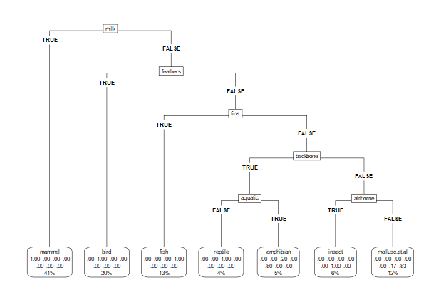
##（3）可视化决策树
treeModelData <- getLearnerModel(tunedTreeModel)
library(rpart.plot)
rpart.plot(treeModelData, roundint = FALSE, type = 5)

2.4 嵌套交叉验证

 1
 2
 3
 4
 5
 6
 7
 8
 9
10
11
12
13
14
15
16
17
18
19


#inner
inner <- makeResampleDesc("CV", iters = 5)
#outer
outer <- makeResampleDesc("CV", iters = 3)

treeWrapper <- makeTuneWrapper("classif.rpart", resampling = inner, 
                              par.set = treeParamSpace, 
                              control = randSearch) 

parallelStartSocket(cpus = 8)
cvWithTuning <- resample(treeWrapper, zooTask, resampling = outer)
parallelStop()

cvWithTuning
# Resample Result
# Task: zooTib
# Learner: classif.rpart.tuned
# Aggr perf: mmce.test.mean=0.1295306
# Runtime: 13.4196

3、bagging与随机森林

集成学习(Ensemble Learning)是指通过训练多个模型，从而在预测时考虑所有模型的预测结果，可减少单模型的方差。可分为bagging, boosting, stacking三种。虽然集成可用于多种机器学习算法，但还是最常应用于基于树的学习器，例如接下来学到的随机森林就是bagging应用于决策树的经典算法。

Bagging, bootstrap aggregating

（1）决定要训练多少个子模型；

（2）对于每个子模型，进行自助法抽样(bootstrap)。即从训练集中有放回的抽样。

（3）根据上述的抽样，训练每一个子模型；

（4）将新数据输入到每个子模型，做出预测；

（5）汇总所有子模型的预测结果，进行最终的预测。

由于训练各个子模型的过程理论上互不干扰，因此当训练非常多的子模型时可应用并行化多线程处理。

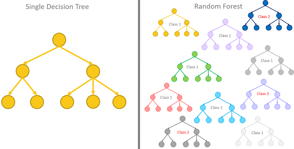
随机森林(Random forest)是Bagging应用于决策树的实现方式。

（1）特征变量抽样：如下图所示，随机森林基于Bagging步骤又多了一步。在上述的第二步结束后，在进行第三步训练每一个决策树时，对特定树的每一个节点都随机选择一定比例的预测变量；然后再从中根据基尼增益选择用于划分的预测变量。

（2）包外(OOB, Out of bag)数据：因为Bagging的自助法抽样，所以每个决策树总会有一些重复样本，而有一定比例的（大部分说法是1/3）样本没有被抽到。换一个角度思考，对于一个样本来说，在随机森林的k个决策树模型中，会有~1/3的决策树训练时没有用到该样本。因此可用来评价、验证模型。

（3）超参数: ①多少个决策树(不考虑计算开销，越多越好)；②在每个节点随机采样的特征数量，即上面第一点的特征变量抽样；③叶节点的最小样本数等与决策树类似的超参数。

（4）降低方差：bagging适合用于决策树算法，因为bagging的集成方法有利于降低不稳定的强学习器base learnner，比如决策树算法一般预测方差很大。

4、随机森林mlr建模

仍使用上面训练决策树所用到的模型

4.1 动物特征训练数据集

 1
 2
 3
 4
 5
 6
 7
 8
 9
10
11
12
13
14
15
16
17
18
19
20
21
22
23
24
25
26
27
28


library(mlr3verse)
library(tidyverse)

data(Zoo, package = "mlbench")
Zoo2 = Zoo %>% 
        dplyr::mutate(across(where(is.logical), as.factor))
str(Zoo2)
# 'data.frame':	101 obs. of  17 variables:
# $ hair    : Factor w/ 2 levels "FALSE","TRUE": 2 2 1 2 2 2 2 1 1 2 ...
# $ feathers: Factor w/ 2 levels "FALSE","TRUE": 1 1 1 1 1 1 1 1 1 1 ...
# $ eggs    : Factor w/ 2 levels "FALSE","TRUE": 1 1 2 1 1 1 1 2 2 1 ...
# $ milk    : Factor w/ 2 levels "FALSE","TRUE": 2 2 1 2 2 2 2 1 1 2 ...
# $ airborne: Factor w/ 2 levels "FALSE","TRUE": 1 1 1 1 1 1 1 1 1 1 ...
# $ aquatic : Factor w/ 2 levels "FALSE","TRUE": 1 1 2 1 1 1 1 2 2 1 ...
# $ predator: Factor w/ 2 levels "FALSE","TRUE": 2 1 2 2 2 1 1 1 2 1 ...
# $ toothed : Factor w/ 2 levels "FALSE","TRUE": 2 2 2 2 2 2 2 2 2 2 ...
# $ backbone: Factor w/ 2 levels "FALSE","TRUE": 2 2 2 2 2 2 2 2 2 2 ...
# $ breathes: Factor w/ 2 levels "FALSE","TRUE": 2 2 1 2 2 2 2 1 1 2 ...
# $ venomous: Factor w/ 2 levels "FALSE","TRUE": 1 1 1 1 1 1 1 1 1 1 ...
# $ fins    : Factor w/ 2 levels "FALSE","TRUE": 1 1 2 1 1 1 1 2 2 1 ...
# $ legs    : int  4 4 0 4 4 4 4 0 0 4 ...
# $ tail    : Factor w/ 2 levels "FALSE","TRUE": 1 2 2 1 2 2 2 2 2 1 ...
# $ domestic: Factor w/ 2 levels "FALSE","TRUE": 1 1 1 1 1 1 2 2 1 2 ...
# $ catsize : Factor w/ 2 levels "FALSE","TRUE": 2 2 1 2 2 2 2 1 1 1 ...
# $ type    : Factor w/ 7 levels "mammal","bird",..: 1 1 4 1 1 1 1 4 4 1 ...

##第1~16列为动物特征
##第17列为动物名标签

4.2 确定预测目标与训练方法

 1
 2
 3
 4
 5
 6
 7
 8
 9
10
11
12
13
14
15
16
17
18
19
20
21
22
23
24


#（1）确定预测目标，根据1~16列数据预测动物类别
task_classif = as_task_classif(Zoo2, target = "type")
task_classif$col_roles$stratum = "type"

#（2）指定随机森林分类算法
learner = lrn("classif.rpart", predict_type="prob")
learner$param_set

#（3）超参数组合以及遍历方法
search_space = ps(
  num.trees = p_int(lower=1,upper=1000),
  mtry = p_int(lower=6,upper=12),
  min.node.size = p_dbl(lower=1, upper=5),
  max.depth = p_int(lower=1,upper=20)
)

design = expand.grid(num.trees=c(300, 500, 1000),
                     mtry=c(6, 9, 12),
                     min.node.size=c(1,2,3,4,5),
                     max.depth = c(3, 6, 9)) %>% as.data.table()

#（4）交叉验证方法与模型评价指标
resampling = rsmp("cv")
measure = msr("classif.acc")

4.3 模型训练优化超参数

 1
 2
 3
 4
 5
 6
 7
 8
 9
10
11
12
13
14
15
16
17
18
19
20
21
22
23
24
25
26
27
28
29
30
31
32
33
34
35
36
37
38
39
40
41
42
43
44


##创建实例
instance = TuningInstanceSingleCrit$new(
  task = task_classif,
  learner = learner,
  resampling = resampling,
  measure = measure,
  terminator = trm("none"),
  search_space = search_space
)
tuner = tnr("design_points", design = design)  
##优化超参数
tuner$optimize(instance)
as.data.table(instance$archive)[,1:5]
#      num.trees mtry min.node.size max.depth classif.acc
#   1:       300    6             1         3   0.9311764
#   2:       500    6             1         3   0.9200653
#   3:      1000    6             1         3   0.9200653
#   4:       300    9             1         3   0.8814005
#   5:       500    9             1         3   0.9004481
#  ---                                                   
# 131:       500    9             5         9   0.9718615
# 132:      1000    9             5         9   0.9718615
# 133:       300   12             5         9   0.9623377
# 134:       500   12             5         9   0.9623377
# 135:      1000   12             5         9   0.9718615

instance$result_learner_param_vals
# $num.threads
# [1] 1

# $num.trees
# [1] 300

# $mtry
# [1] 12

# $min.node.size
# [1] 4

# $max.depth
# [1] 6
instance$result_y
#classif.acc 
#0.9813853

4.4 使用最佳超参数建模

 1
 2
 3
 4
 5
 6
 7
 8
 9
10
11
12
13
14
15
16
17
18
19
20
21
22
23
24
25
26
27
28
29
30
31
32
33
34
35


learner$param_set$values = instance$result_learner_param_vals
learner$train(task_classif)
learner$model
# Ranger result

# Call:
#  ranger::ranger(dependent.variable.name = task$target_names, data = task$data(),      probability = self$predict_type == "prob", case.weights = task$weights$weight,      num.threads = 1L, num.trees = 300L, mtry = 12L, min.node.size = 4L,      max.depth = 6L) 

# Type:                             Probability estimation 
# Number of trees:                  300 
# Sample size:                      101 
# Number of independent variables:  16 
# Mtry:                             12 
# Target node size:                 4 
# Variable importance mode:         none 
# Splitrule:                        gini 
# OOB prediction error (Brier s.):  0.04122035 


predict(learner$model, task_classif)
prediction = learner$predict(task_classif)
prediction$confusion
#                truth
# response        mammal bird reptile fish amphibian insect mollusc.et.al
#   mammal            41    0       0    0         0      0             0
#   bird               0   20       0    0         0      0             0
#   reptile            0    0       5    0         0      0             0
#   fish               0    0       0   13         0      0             0
#   amphibian          0    0       0    0         4      0             0
#   insect             0    0       0    0         0      8             0
#   mollusc.et.al      0    0       0    0         0      0            10

prediction$score(msrs(c("classif.acc","classif.ce")))
# classif.acc  classif.ce 
# 1           0 

1、决策树基础#

1.1 决策树的构成#

1.2 基尼系数#

1.3 防止决策树过拟合#

2、决策树mlr建模#

2.1 动物特征数据集#

2.2 确定预测目标与训练方法#

2.3 模型训练#

2.4 嵌套交叉验证#

3、bagging与随机森林#

4、随机森林mlr建模#

4.1 动物特征训练数据集#

4.2 确定预测目标与训练方法#

4.3 模型训练优化超参数#

4.4 使用最佳超参数建模#