R包NMF非负矩阵分解

 1
 2
 3
 4
 5
 6
 7
 8
 9
10
11
12
13

# 模拟数据：100个样本的30个基因表达矩阵
set.seed(42)
exp_mat = matrix(abs(rnorm(3000)), nrow = 30) 
colnames(exp_mat) = paste0("sp",1:100)
rownames(exp_mat) = paste0("gene",1:30)
dim(exp_mat)
# [1]  30 100
exp_mat[1:4,1:4]
#             sp1       sp2       sp3       sp4
# gene1 1.3709584 0.4554501 0.3672346 1.3921164
# gene2 0.5646982 0.7048373 0.1852306 0.4761739
# gene3 0.3631284 1.0351035 0.5818237 0.6503486
# gene4 0.6328626 0.6089264 1.3997368 1.3911105

 1
 2
 3
 4
 5
 6
 7
 8
 9
10
11
12
13
14
15
16
17
18
19
20
21
22
23
24
25
26
27
28
29

library(NMF)

# 支持算法：c("brunet","lee","ls-nmf","nsNMF","offset","pe-nmf","snmf/r","snmf/l") 
nmf_model <- nmf(exp_mat, rank = 3, method = "brunet", seed = 42)

# 获取基矩阵（基因--细胞）
basis_matrix <- basis(nmf_model)
dim(basis_matrix)
# [1] 30  3
head(basis_matrix)
#            [,1]      [,2]      [,3]
# gene1 1.7436283 0.7842223 3.0718832
# gene2 1.0542018 0.9599996 2.8275129
# gene3 2.7498596 1.4277110 1.0828163
# gene4 0.8918389 1.8432274 2.7861665
# gene5 4.2662810 0.8883752 0.3467359
# gene6 5.8054591 0.6420813 0.2967837

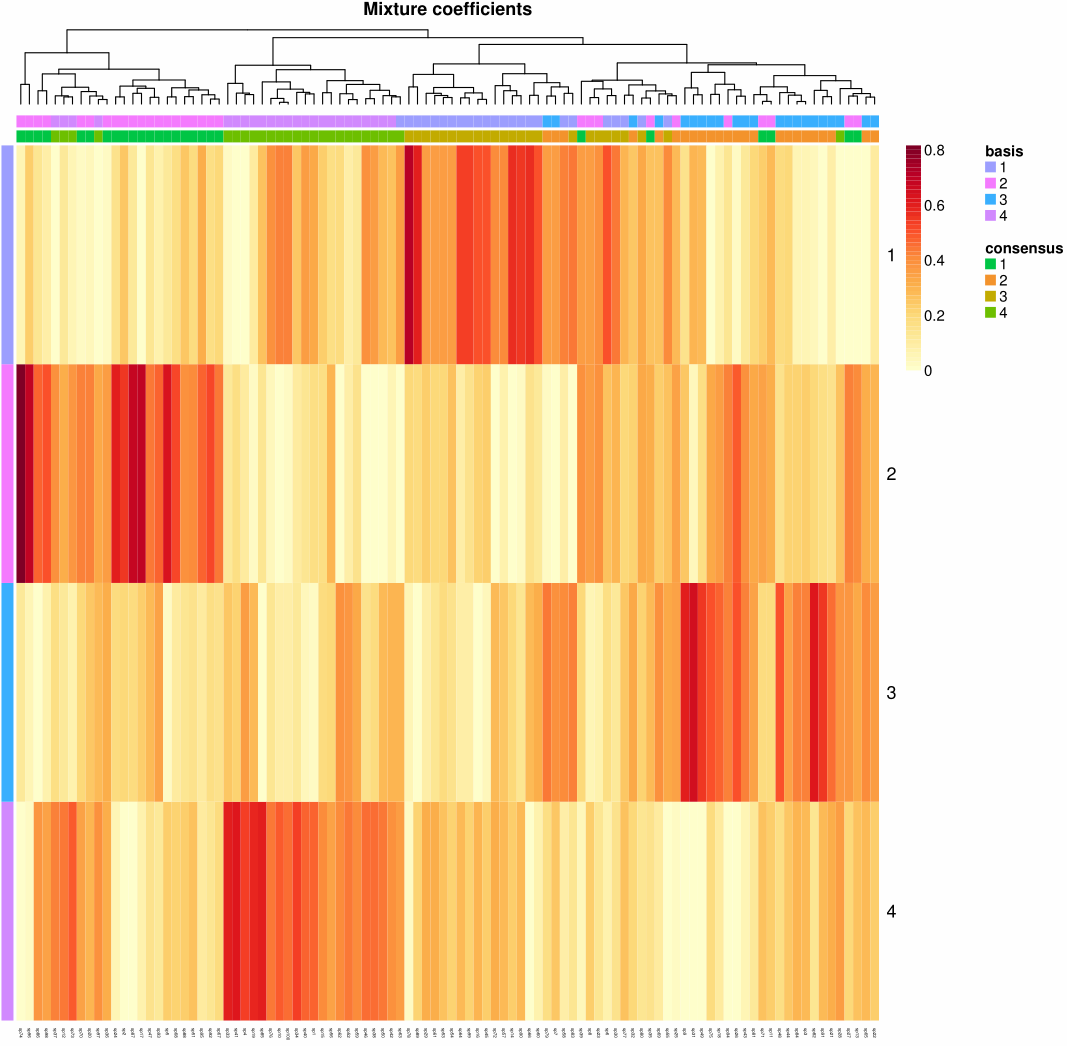
# 获取系数矩阵（细胞--样本）
coef_matrix <- coef(nmf_model)
dim(coef_matrix)
# [1]   3 100
head(coef_matrix[,1:3])
#              sp1        sp2        sp3
# [1,] 0.002897117 0.02866644 0.02137146
# [2,] 0.131645724 0.14692969 0.04635707
# [3,] 0.022945508 0.05598917 0.11973042
# [4,] 0.169223269 0.06491003 0.13558182
# [5,] 0.088389864 0.10569255 0.12587923

1
2
3
4
5
6

# 遍历2~10种候选值，每个重复10次
nmf_model_candi <- nmf(exp_mat, rank = 2:10, method = "brunet", nrun=10)

pdf("candi_ranks.pdf", width=8, height=8)
plot(nmf_model_candi)
dev.off()

1
2
3

pdf("candi_ranks_consensusmap.pdf", width=10, height=10)
consensusmap(nmf_model_candi)
dev.off()

1
2
3

nmf_model = nmf(exp_mat, rank = 4, method = "brunet", nrun=100)
basis_matrix <- basis(nmf_model) 
coef_matrix <- coef(nmf_model)   

1
2
3

pdf("basismap.pdf", width = 10, height = 10)
basismap(nmf_model)
dev.off()

1
2
3

pdf("coefmap.pdf", width = 10, height = 10)
coefmap(nmf_model)
dev.off()

1
2
3

pdf("consensusmap.pdf", width = 10, height = 10)
consensusmap(nmf_model, labCol=NA, labRow=NA)
dev.off()

1
2
3
4
5
6

set.seed(42)
V = matrix(abs(rnorm(50)), nrow =5)
set.seed(42)
W = matrix(abs(rnorm(20)), nrow =5)
set.seed(42)
H = matrix(abs(rnorm(40)), nrow =4)

1
2
3
4

nmf_obj <- nmf(V, 4,  W = W, method = "brunet", nrun = 100)
fit(nmf_obj)
H2 <- coef(nmf_obj)
H2[,1:4]

1
2
3
4

nmf_obj <- nmf(V, 4,  H = H, method = "brunet", nrun = 100)
fit(nmf_obj)
W2 <- coef(nmf_obj)
W2[,1:4]