MuSiC包根据scRNAseq预测Bulk细胞组成

MuSiC(MUlti-Subject SIngle Cell deconvolution)是来自宾夕法尼亚大学Biostatistics, Epidemiology and Informatics系的Mingyao Li课题组于2019年发表于Nature Communication的一个工具R包，可根据单细胞转录组信息推测Bulk RNA-seq细胞组成。而后，该团队又于2022年在Briefing in bioinformatics发表了扩展版本MuSiC2，可以考虑更复杂的场景。

Paper–MuSic：https://doi.org/10.1038/s41467-018-08023-x

Paper–MuSic2：https://doi.org/10.1093/bib/bbac430

Github：https://xuranw.github.io/MuSiC/index.html

1、算法简介

1.1 MuSiC

如下是流程图，由于单细胞数据一般存在多个样本，MuSiC的核心是“marker gene consistency”，即基因的表达一致性体现在同种细胞类型间(cross cell)，也体现在不同样本间(cross subject)。在去卷积注释时针对这些基因会赋予较高的权重。
另一方面考虑到，作者认为Solid tissues often contain closely related cell types，即一般算法难以对这些类似的细胞进行区分。对此，MuSiC分两步预测。首先进行general prediction，然后针对每个cluster分别单独预测具体的细胞类型比例。

1.2 MuSiC2

MuSiC2算法在上述基础考虑到Bulk RNAseq的组间差异带来的影响。一般单细胞数据来自健康人组织，而Bulk RNAseq可能有健康，疾病等多组。
作者认为需要避免健康与疾病组间的差异基因表达对细胞类型去卷积产生的干扰，即选择stable genes对疾病组样本注释(删去组间细胞类型差异表达基因)。

2、R包用法

1
2
3
4
5
6
7
8


# 安装
# BiocManager::install("TOAST")
devtools::install_github('xuranw/MuSiC')

## 参考Github教程提前下载示例数据
# Bulk data为ExpressionSet格式
# scRNA-seq data为SingleCellExperiment format格式
# 表达矩阵均为原始read counts，不需要标准化

2.1 MuSiC简单用法

 1
 2
 3
 4
 5
 6
 7
 8
 9
10
11
12
13
14
15
16
17
18
19
20
21
22
23
24
25
26
27
28
29
30
31
32
33
34
35
36
37
38
39
40
41
42


# (1) Bulk data
GSE50244.bulk.eset = readRDS('./GSE50244bulkeset.rds')
dim(GSE50244.bulk.eset)
# Features  Samples 
# 32581       89 
bulk.mtx = exprs(GSE50244.bulk.eset)

# (2) scRNA-seq data
EMTAB.sce = readRDS('./EMTABsce_healthy.rds')
dim(EMTAB.sce)
# [1] 25453  1097
# 主要需要两列注释信息：样本名与细胞类型
table(EMTAB.sce$cellType, EMTAB.sce$sampleID)

#                          1   2   4   5   6   8
# acinar                   4  20   3  80   3   2
# alpha                   28 117  92  26 136  44
# beta                    12  48  35  32  34  10
# co-expression            3   3   6   5   6   3
# delta                    7  21  12   2   7  10
# ductal                   4  19  14  67   8  23
# endothelial              1   1   8   0   1   2
# epsilon                  0   1   3   1   0   0
# ......

# (3) Estimate cell type proportions
music_pred_obj = music_prop(bulk.mtx = bulk.mtx, # bulk exp
                            sc.sce = EMTAB.sce, # scRNAseq obj
                            clusters = 'cellType',  # cluster column
                            samples = 'sampleID',   # sample  column
                            select.ct = c('alpha', 'beta', 'delta', 
                                          'gamma', 'acinar', 'ductal'), 
                            verbose = F)
names(music_pred_obj)
# [1] "Est.prop.weighted" "Est.prop.allgene"  "Weight.gene"       "r.squared.full"    "Var.prop"      
## 前两者分别表示MuSiC与NNLS算法的结果：每个样本(行)对于每种细胞类型(列)的比例，并进行样本水平归一化
music_pred_obj$Est.prop.weighted[1:4,]
#          alpha      beta       delta        gamma     acinar    ductal
# Sub1 0.2079168 0.1746030 0.002203054 0.0015887041 0.09597685 0.5177117
# Sub2 0.6964173 0.1197928 0.003683287 0.0007471486 0.03078049 0.1485789
# Sub3 0.1913485 0.3521117 0.032037770 0.0003117540 0.19143687 0.2327533
# Sub4 0.2339358 0.4673282 0.009425930 0.0226075392 0.05385258 0.2128500

2.2 MuSiC分步预测

即针对细胞类型相似的Bulk组织类型（Solid tissues often contain closely related cell types）

（1）预处理

 1
 2
 3
 4
 5
 6
 7
 8
 9
10
11
12
13
14


Mouse.bulk.eset = readRDS('./Mousebulkeset.rds')
Mouse.bulk.eset
# 10 19033

Mousesub.sce = readRDS('./Mousesub_sce.rds')
Mousesub.sce
# 10000 16273

Mousesub.basis = music_basis(Mousesub.sce, 
                             clusters = 'cellType', 
                             samples = 'sampleID', 
                             select.ct = c('Endo', 'Podo', 'PT', 'LOH', 'DCT', 
                                           'CD-PC', 'CD-IC', 'Fib','Macro', 
                                           'Neutro','B lymph', 'T lymph', 'NK'))

（2）根据单细胞的标签定义相似的细胞组

 1
 2
 3
 4
 5
 6
 7
 8
 9
10
11
12
13
14
15
16
17


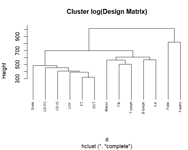
d <- dist(t(log(Mousesub.basis$Disgn.mtx + 1e-6)), method = "euclidean")
# d <- dist(t(log(Mousesub.basis$M.theta + 1e-8)), method = "euclidean")
hc1 <- hclust(d, method = "complete" )
plot(hc1, cex = 0.6, hang = -1, main = 'Cluster log(Design Matrix)')

clusters.type = list(C1 = 'Neutro', 
                     C2 = 'Podo', 
                     C3 = c('Endo', 'CD-PC', 'LOH', 'CD-IC', 'DCT', 'PT'), 
                     C4 = c('Macro', 'Fib', 'B lymph', 'NK', 'T lymph'))

# 添加到单细胞数据中
cl.type = as.character(Mousesub.sce$cellType)
for(cl in 1:length(clusters.type)){
  cl.type[cl.type %in% clusters.type[[cl]]] = names(clusters.type)[cl]
}
Mousesub.sce$clusterType = factor(cl.type, 
                                  levels = c(names(clusters.type), 'CD-Trans', 'Novel1', 'Novel2'))

（3）鉴定每大组内的组间marker基因(marker genes within each group)

1
2
3
4
5
6
7
8
9


load('./IEmarkers.RData')
IEmarkers = list(NULL, NULL, Epith.marker, Immune.marker)
names(IEmarkers) = c('C1', 'C2', 'C3', 'C4')
str(IEmarkers)
# List of 4
#  $ C1: NULL
#  $ C2: NULL
#  $ C3: chr [1:2614] "Rp1" "Sox17" "1700034P13Rik" "Prex2" ...
#  $ C4: chr [1:8126] "Sox17" "Gm37988" "Gm26901" "Mybl1" ...

（4）Estimate cell type proportions

 1
 2
 3
 4
 5
 6
 7
 8
 9
10
11
12
13
14
15


music_pred_obj = music_prop.cluster(bulk.mtx = exprs(Mouse.bulk.eset), 
                                    sc.sce = Mousesub.sce, 
                                    group.markers = IEmarkers, 
                                    clusters = 'cellType', 
                                    groups = 'clusterType', 
                                    samples = 'sampleID', 
                                    clusters.type = clusters.type)
dim(music_pred_obj$Est.prop.weighted.cluster)
# 10, 13
music_pred_obj$Est.prop.weighted.cluster[1:4, 1:4]
#               Neutro        Podo       Endo      CD-PC
# control.NA.27      0 0.009505281 0.04474493 0.02680222
# control.NA.30      0 0.021948575 0.04305809 0.02687187
# control.NA.39      0 0.005628454 0.04412269 0.02802505
# control.NAP.3      0 0.018769776 0.04305809 0.02655007

2.3 MuSiC2用法

 1
 2
 3
 4
 5
 6
 7
 8
 9
10
11
12
13
14
15
16
17
18
19
20
21
22
23
24
25
26
27
28
29


# (1) 50个对照与50个疾病，共100个样本的Bulk data
benchmark.eset = readRDS("./bulk-eset.rds")
benchmark.eset
table(benchmark.eset$group)
# healthy     t2d 
#      50      50

# (2) 来自健康样本的scRNA-seq Data
seger.sce = readRDS("./EMTABsce_healthy.rds")
seger.sce

# (3) Estimate cell type proportions
music2_pred_obj = music2_prop(bulk.control.mtx = bulk.control.mtx, 
                                           bulk.case.mtx = bulk.case.mtx, 
                                           sc.sce = seger.sce, 
                                           clusters = 'cellType', 
                                           samples = 'sampleID', 
                                           select.ct = c('acinar','alpha','beta','delta','ductal','gamma'), 
                                           n_resample=20, sample_prop=0.5,
                                           cutoff_c=0.05,cutoff_r=0.01)
dim(music2_pred_obj$Est.prop)
# [1] 100   6
#         acinar      alpha      beta       delta     ductal       gamma
# 1  0.154031473 0.03854683 0.5124088 0.001545064 0.29346786 0.000000000
# 10 0.559249172 0.13773168 0.2220337 0.005554692 0.07290038 0.002530353
# 12 0.062448310 0.57696213 0.1321646 0.000000000 0.22842496 0.000000000
# 14 0.113631970 0.34670271 0.3154881 0.000000000 0.16988614 0.054291121
# 17 0.078927767 0.31450931 0.2647605 0.000000000 0.34180242 0.000000000
# 2  0.008209709 0.41839211 0.1390657 0.019564262 0.41476824 0.000000000

1、算法简介#

1.1 MuSiC#

1.2 MuSiC2#

2、R包用法#

2.1 MuSiC简单用法#

2.2 MuSiC分步预测#

2.3 MuSiC2用法#

1、算法简介

1.1 MuSiC

1.2 MuSiC2

2、R包用法

2.1 MuSiC简单用法

2.2 MuSiC分步预测

2.3 MuSiC2用法