ClusterGVis包绘制基因表达矩阵热图

 1
 2
 3
 4
 5
 6
 7
 8
 9
10
11
12
13
14

devtools::install_github("junjunlab/ClusterGVis")
packageVersion("ClusterGVis")
# [1] ‘0.0.8’

library(ClusterGVis)
# 示例数据:标准化的 tpm/fpkm/rpkm 表达矩阵
data(exps)
dim(exps)
# [1] 3767    6
head(exps,3)
#           zygote  t2.cell  t4.cell  t8.cell   tmorula blastocyst
# Oog4   1.3132282 1.237078 1.325978 1.262073 0.6549312  0.2067114
# Psmd9  1.0917337 1.315989 1.174417 1.064756 0.8685598  0.4845448
# Sephs2 0.9859232 1.201026 1.123076 1.084673 0.8878931  0.7174088

 1
 2
 3
 4
 5
 6
 7
 8
 9
10
11
12

# (1)确定合适的聚类数
getClusters(exp = exps)

# (2)两种聚类方式 c("mfuzz","kmeans")
cm <- clusterData(exp = exps,
                  cluster.method = "mfuzz", 
                  cluster.num = 8,
                  # subcluster = 1:6, #保留其中的1-6群
                  seed = 42)
table(cm$long.res$cluster)
#    1    2    3    4    5    6    7    8 
# 1590 5532 2070 5310 2418 2538 1680 1464

1
2
3
4
5
6
7

# 一条线代表一个基因
visCluster(object = cm,
       plot.type = "line") #左
visCluster(object = cm,
       plot.type = "line",
       ms.col = c("green","orange","red"),
       add.mline = FALSE) #右

 1
 2
 3
 4
 5
 6
 7
 8
 9
10
11
12
13
14
15
16
17
18
19
20
21
22

pdf("tmp1.pdf", width=8, height=10)
visCluster(object = cm,
           plot.type = "heatmap")

dev.off() # 左

pdf("tmp2.pdf", width=8, height=10,onefile=FALSE)
markGenes = rownames(exps)[sample(1:nrow(exps),30,replace = F)]
visCluster(object = cm,
           plot.type = "heatmap",
           show_row_dend = F,                 #不显示聚类树
           column_names_rot = 45,             #列标题角度
           annnoblock.text = F,               #行注释块不显示基因数量
           ctAnno.col = ggsci::pal_npg()(8),  #行注释块颜色
           markGenes = markGenes,             #注释部分基因名
           genes.gp = c('italic',fontsize = 12), #基因名显示格式
           cluster.order = c(1:9),       # 行clster的顺序
           # sample.group = rep(c("group1","group2","group3"),each = 2),  #添加样本分组
           # sample.col = rep(ggsci::pal_aaas()(3), each=2), 
           sample.order = colnames(exps) # 列sample的顺序
           ) 
dev.off() # 右

 1
 2
 3
 4
 5
 6
 7
 8
 9
10
11
12
13
14
15
16
17

# 热图+线图
pdf("tmp1.pdf", width=8, height=10)
visCluster(object = cm,
           plot.type = "both",
           show_row_dend = F,
           textbox.size = 5,
           annnoblock.text = F)
dev.off()

# 热图+箱图
pdf("tmp2.pdf", width=8, height=10)
visCluster(object = cm,
           plot.type = "both",
           add.box = T,
           add.line = F,
           boxcol = ggsci::pal_npg()(8))
dev.off()

 1
 2
 3
 4
 5
 6
 7
 8
 9
10
11
12
13
14
15
16
17
18
19
20
21
22
23
24
25
26
27
28
29
30
31
32

head(termanno)	
#   id                               term
# 1 C1              developmental process
# 2 C1   anatomical structure development
# 3 C1 multicellular organism development
pdf("tmp1.pdf", width=8, height=10)
visCluster(object = cm,
           plot.type = "both",
           show_row_dend = F,
           annoTerm.data = termanno,
           line.side = "left")
dev.off()

head(termanno2, 3)
#   id                               term     pval
# 1 C1              developmental process 3.17e-69
# 2 C1   anatomical structure development 1.44e-68
# 3 C1 multicellular organism development 1.36e-66
pdf("tmp2.pdf", width=12, height=10)
visCluster(object = ck,
           plot.type = "both",
           annoTerm.data = termanno2,
           line.side = "left", #线图设置在左侧
           show_row_dend = F,  #不显示聚类层级图
           go.col = rep(ggsci::pal_d3()(8),each = 3),  #直接指定颜色
           go.size = "pval",    #大小映射P值
           add.bar = T, textbar.pos = c(0.8,0.2),
           annoTerm.mside = "left" # 增加条形图表示通路的P值， -log10转换 
           # sample.order = rev(colnames(exps)),  # 指定样本你顺序
           # subgroup.anno = c("C4","C6","C8")  #只针对亚群注释
           )
dev.off()

 1
 2
 3
 4
 5
 6
 7
 8
 9
10
11
12
13
14

library(Seurat)
sce = pbmc3k.SeuratData::pbmc3k
sce$celltype = as.character(sce$seurat_annotations)
Idents(sce) = "celltype"
deg_wilcox =  Seurat::FindAllMarkers(sce,
                               only.pos = TRUE,
                               min.pct = 0.25,
                               logfc.threshold = 0.25)
deg_wilcox_top = deg_wilcox %>%
  dplyr::group_by(cluster) %>%
  dplyr::top_n(n = 20, wt = avg_log2FC)
table(deg_wilcox_top$cluster)
# Memory CD4 T            B   CD14+ Mono           NK        CD8 T  Naive CD4 T FCGR3A+ Mono           DC     Platelet 
#           20           20           20           20           20           20           20           20           20

 1
 2
 3
 4
 5
 6
 7
 8
 9
10
11
12
13
14
15
16

# [1] 以细胞群的均值作为输入,且默认对基因进行去重
st.data1 <- prepareDataFromscRNA(object = sce,
                                diffData = deg_wilcox_top,
                                showAverage = TRUE)

# [2] 不对基因进行去重处理，添加后缀
st.data2 <- prepareDataFromscRNA(object = sce,
                                diffData = deg_wilcox_top,
                                showAverage = TRUE,
                                keep.uniqGene = FALSE,
                                sep = "_")  #"gene_1","gene_2",....

# [3] 以每个细胞单独的表达作为输入
st.data3 <- prepareDataFromscRNA(object = sce,
                                diffData = deg_wilcox_top,
                                showAverage = FALSE)

 1
 2
 3
 4
 5
 6
 7
 8
 9
10
11
12
13
14

# 这里使用该包自带的GO富集方法
library(org.Hs.eg.db)
enrich <- enrichCluster(object = st.data,
                        OrgDb = org.Hs.eg.db,
                        type = "BP",
                        organism = "hsa",
                        pvalueCutoff = 0.5,
                        topn = 3,
                        seed = 5201314)
head(enrich, 3)
#                group                      Description       pvalue    ratio
# GO:0002181...1    C1          cytoplasmic translation 1.318764e-10 36.84211
# GO:1903131        C1 mononuclear cell differentiation 4.891104e-06 31.57895
# GO:0030217        C1           T cell differentiation 8.839690e-06 26.31579

 1
 2
 3
 4
 5
 6
 7
 8
 9
10
11
12
13
14
15
16
17
18
19
20
21
22

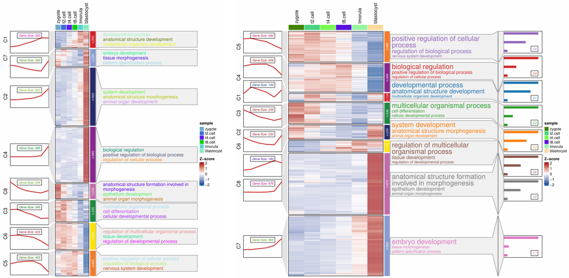
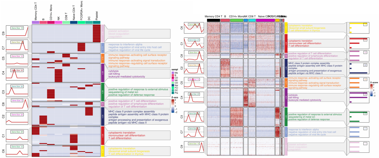
pdf('tmp1.pdf',height = 10,width = 12,onefile = F)
visCluster(object = st.data1,
           plot.type = "both",
           show_row_dend = F,
           markGenes.side = "left",
           annoTerm.data = enrich,
           line.side = "left",
           go.col = rep(jjAnno::useMyCol("stallion",n = 9),each = 3))
dev.off()

pdf('tmp2.pdf',height = 10,width = 14,onefile = F)
visCluster(object = st.data3,
           plot.type = "both",
           show_row_dend = F,
           markGenes.side = "left",
           annoTerm.data = enrich,
           line.side = "left",
           go.col = rep(jjAnno::useMyCol("stallion",n = 9),each = 3),
           add.bar = T, 
           annoTerm.mside = "left", 
           show_column_names = F)
dev.off()