WGCNA基因加权共表达网络分析

1、关于WGCNA原理

1.1 建立共表达网络

在基因共表达网络中，节点node代表基因，边edge代表两个基因间共表达关系。

若一个基因同时与多个基因存在相关性，称为hub基因。
若一群基因存在高度互相相关，称为module。

基因共表达网络的展示形式一般为 n × n 邻接矩阵adjacency matrix(n个基因)

（1）similarity matrix

在得到一个m × n 表达矩阵（m个样本，n个基因）后，第一步是计算两基因在多样本的表达水平相关性（例如spearman correlation，值一般在-1 ~ 1之间），从而得到表达相似度矩阵similarity matix，简记为S。根据是否考虑相关性的正负性，有两种处理方式。 $$ S=[s_{ij}], \quad s_{ij} = |cor(i,j)| \quad if ‘unsign’ $$

$$ S=[s_{ij}], \quad s_{ij} = \frac{1+cor(i,j)}{2} \quad if ‘sign’ $$

不要把sign和directed弄混了。前者表示相关的正负性，后者表示方向性。使用WGCNA建立的都是undirected网络。

（2）adjacency matrix

第二步是使用adjacency function将基因表达相似矩阵转为共表达邻接矩阵。根据adjacency function的特点分为hard与soft两种。

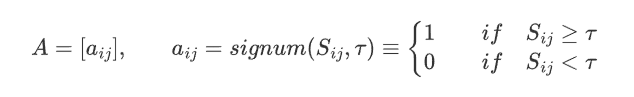
Hard adjacency function：设置一个阈值，若相关性高于阈值，则认为存在共表达关系，记为1；反之，则不存在，记为0。由此得到的结果成为 Unweighted Network。

该网络中每个节点的连接度(connectivity)即为共表达的基因数。

此方法的关键是确定一个合理阈值。对此最显著的弊端是假设定义0.8为阈值，为什么0.79就认为不存在共表达关系呢。

1
2
3
4
5
6


$$
A=[a_{ij}], && a_{ij}=signum(S_{ij}, \tau)  \equiv \begin{cases}
1 && if & S_{ij}\geq \tau \\
0 && if & S_{ij}< \tau 
\end{cases}
$$

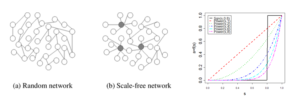
Soft adjacency function：使用的前提是假设基因共表达网络为scale-free netork无尺度网络，其特征是少部分节点具有高连通性，大部分节点具有低连通性。在该网络中所有edge中，大部分接近于0，小部分接近于1，符合幂律分布，可使用幂函数(power function)拟合。由此得到的结果位于[0,1]之间，成为Weighted Network。

该网络中每个节点的连接度(connectivity)即为所有邻居基因的共表达权重总和。

此方法的关键是确定一个合理指数，使得符合幂律分布。由于更符合生物网络的本质，因此推荐使用这种方法。

$$ A=[a_{ij}], \quad a_{ij}=power(s_{ij},\beta)\equiv|s_{ij}|^{\beta} $$

Scale-free network有两个特点

（1）对节点error有一定容忍度，即破坏其中普通的低连通性节点，不会影响整体网络结构；

（2）一旦是少数的hub node发生错误，则会造成严重后果。

（3）topological overlap matrix

在WGCNA中，为了minimize effects of noise and spurious associations 将上一步得到adjacency matrix，转化为 topological overlap matrix (TOM)。这一转换主要是考虑到了其它基因对于两两基因间共表达关系的贡献。 $$ k_i=\sum_{u}a_{iu} \tag{1} $$

$$ l_{ij}=\sum_{u}a_{iu}a_{uj} \tag{2} $$

$$ \Omega=[w_{ij}], \quad w_{ij} = \frac{l_{ij} + a_{ij}}{min{k_i,k_j} + 1 - a_{ij}} \tag{3} $$

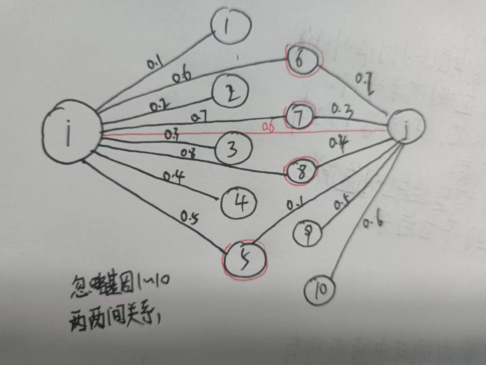
对于式1，计算基因的连通性connectivity；对于式2，计算基因i与基因j分别与其余所有基因共表达指标乘积的和。

举例来说基因i与基因j之间的共表达值为0.6，

基因i与基因1~8的共表达值分别为0.1~0.8 → ki=3.6

基因j与基因5~10的共表达值分别为0.1~0.6 → kj=1.8

基因i与基因j存在3个共同令居，故 lij=(0.5*0.1)+(0.6*0.2)+(0.7*0.3)=0.38

所以wij = (0.38 + 0.6)/(1.8+1-0.6) = 0.445

由原来的0.6变为了0.445，降低的原因在于第三方基因与这对基因的相关性并不一致。

1.2 鉴定模块及相关分析

鉴定模块Module：将基因共表达网络转化为 dissimilarity matrix（1-TOM），然后基于树状图的层次聚类进行动态剪切将基因划分为若干模块。
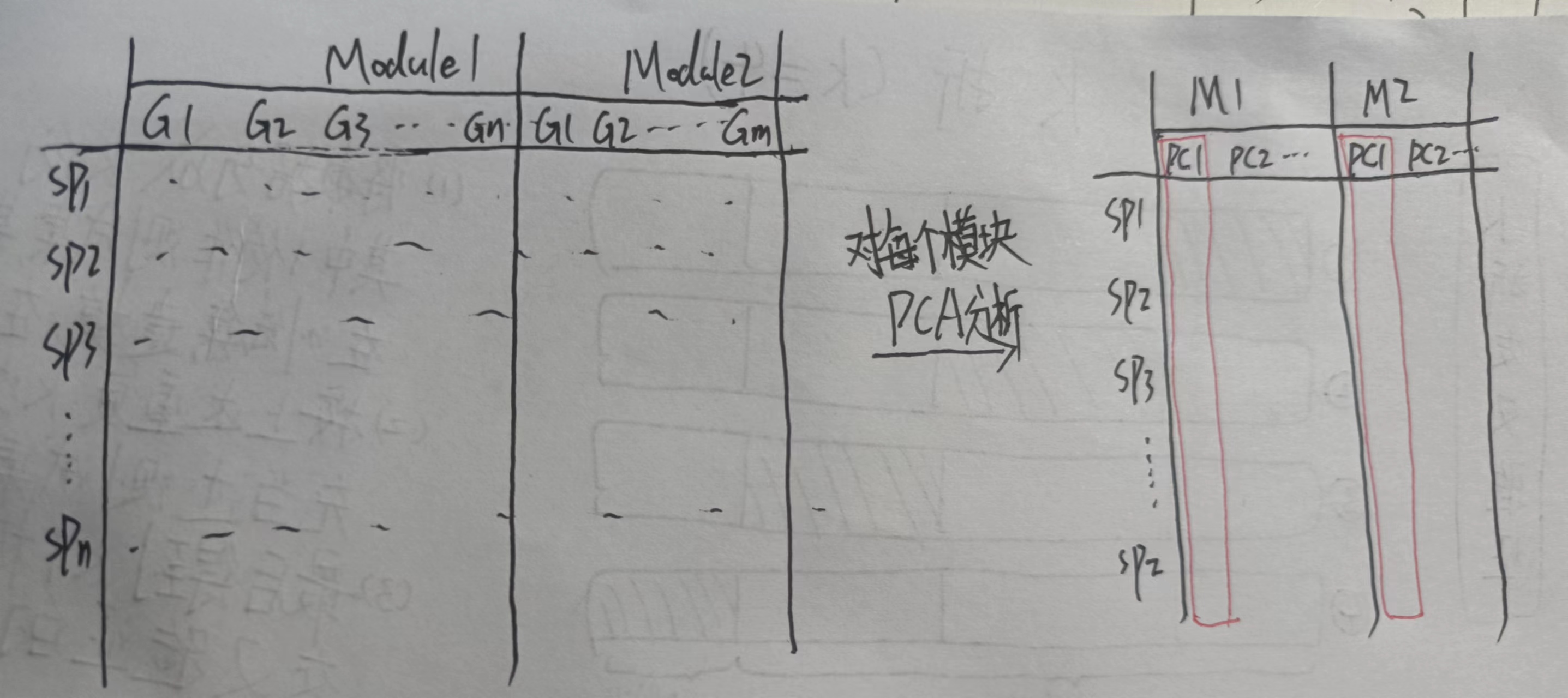
Module eigengene模块特征值：即使用一个特征值代表某样本对于某个模块的特征Trait情况。具体计算方法是使用主成分分析PCA，提取第一个主成分值，如下图所示。

Gene significance，GS：即比较样本基因表达与样本表型之间的相关性，有如下两种计算方式。一种是计算相关性绝对值，另一种是计算相关显著性。
- 总体原则是GS越接近1，表示基因与表型越相关。

$$ \begin{align} & GS_i = |cor(x_i,T)| \tag{1} \ & GS_i = -log,p_i \tag{2} \ \end{align} $$

Module significance，MS：即模块内基因的平均GS

$$ MS_{blue} = \frac{\sum_{i=1}^{n}GS_i}{n} $$

Module Membership: 模块内基因表达与模块特征值的相关性，也称为eigengene-based connectivity，KME。
- 其绝对值越接近1，表明与该模块相关。

$$ MM^{blue}(i)=K_{cor,i}^{blue}=cor(x_i, E^{blue}) $$

Intramodular connectivity模块内连通性：表示某基因与某个模块内基因的共表达权重关系总和。

参考资料： [1] A General Framework for Weighted Gene Co-Expression Network Analysis. doi:10.2202/1544-6115.1128

[2] WGCNA: an R package for weighted correlation network analysis. doi:10.1186/1471-2105-9-559

2、WGCNA实操

以下代码、数据主要参考官方教程

1
2


# BiocManager::install("WGCNA")
library(WGCNA)

2.1 整理输入数据

关于WGCNA的输入数据要求，官方文档已经做说明，大致如下几点：

（1）至少20个样本以上，越多越好；

（2）可以过滤点低表达或者低方差的基因，以减少干扰信息。但不太建议直接使用差异基因。

（3）WGCNA最初用于芯片测序数据，也适用于RNA-seq数据。关于RNAseq标准化，由于不涉及到不同基因之间的比较，所有常规标准化方式都可以。

整理表达矩阵

 1
 2
 3
 4
 5
 6
 7
 8
 9
10
11
12
13
14
15
16
17
18
19
20
21
22
23
24
25
26
27
28
29
30
31
32
33
34
35
36


exp_dat = read.csv("LiverFemale3600.csv",row.names = 1) %>% .[,-c(1:7)]
# [1] 3600  135
##(1)转置为行名为样本，列名为基因的表达矩阵
exp_mt = as.data.frame(t(exp_dat))
exp_mt[1:4,1:4]
#       MMT00000044 MMT00000046 MMT00000051 MMT00000076
# F2_2    -1.81e-02     -0.0773     -0.0226    -0.00924
# F2_3     6.42e-02     -0.0297      0.0617    -0.14500
# F2_14    6.44e-05      0.1120     -0.1290     0.02870
# F2_15   -5.80e-02     -0.0589      0.0871    -0.04390


##(2)判断数据质量--缺失值
gsg = goodSamplesGenes(exp_mt)
gsg$allOK
# [1] TRUE


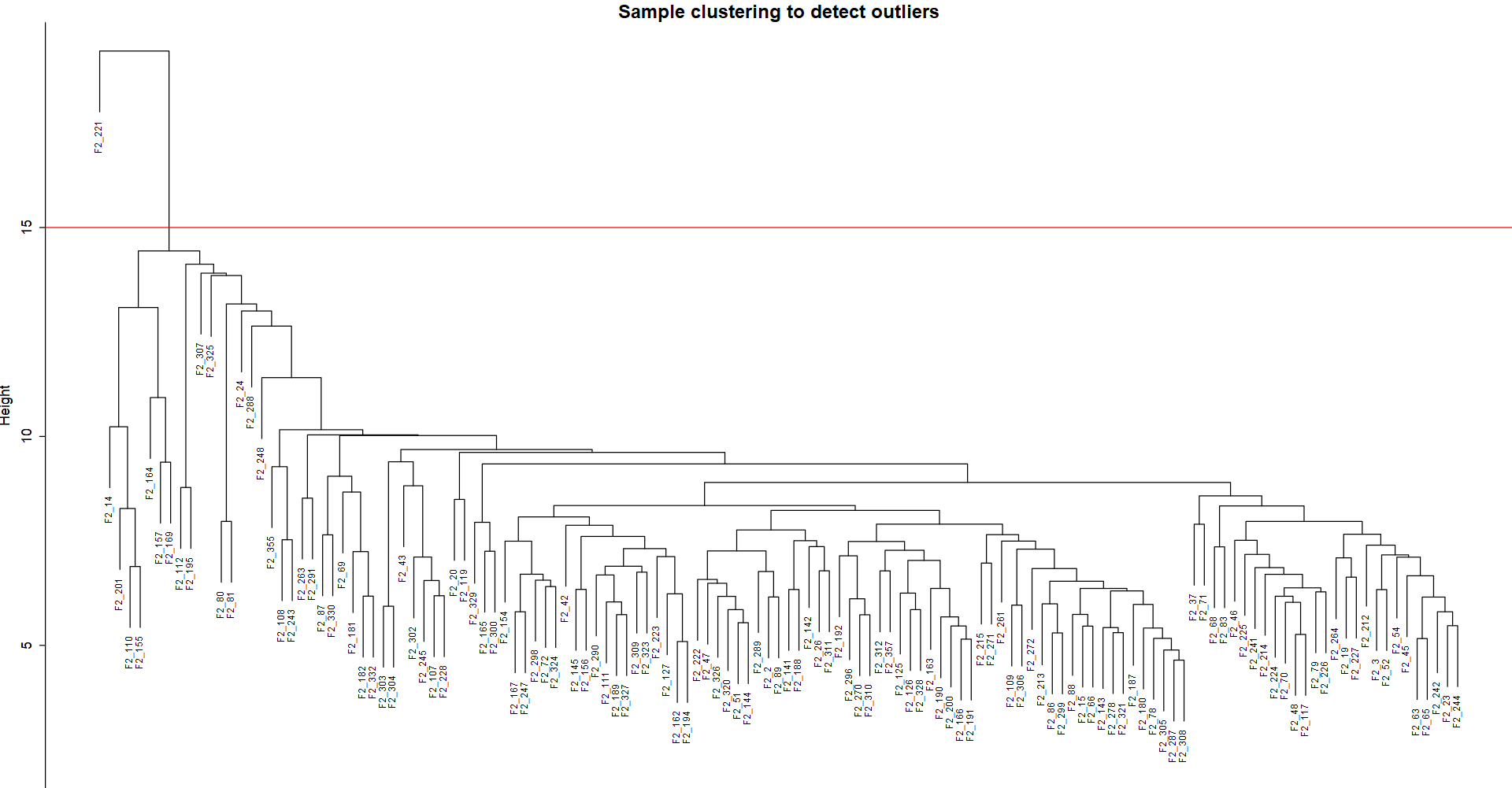
##(3)判断数据质量--离群点样本
sampleTree = hclust(dist(exp_mt), method = "average")
sizeGrWindow(12,9)
par(cex = 0.6);
par(mar = c(0,4,2,0))
plot(sampleTree, main = "Sample clustering to detect outliers", 
     sub="", xlab="", cex.lab = 1.5,
     cex.axis = 1.5, cex.main = 2)
abline(h = 15, col = "red") #根据实际情况而定

##如下图所示，存在一个显著离群点；剔除掉
clust = cutreeStatic(sampleTree, cutHeight = 15, minSize = 10)
table(clust)
# clust
# 0   1 
# 1 134 
keepSamples = (clust==1)
exp_mt_f = exp_mt[keepSamples, ]

整理样本表型数据

 1
 2
 3
 4
 5
 6
 7
 8
 9
10
11
12
13
14
15
16
17
18
19
20
21
22


trait_dat = read.csv("ClinicalTraits.csv",row.names = 2) %>% 
  .[,setdiff(11:37,c(15,30))]
trait_dat_f = trait_dat[rownames(exp_mt_f),]
#       length_cm ab_fat other_fat total_fat
# F2_2       10.5   3.81      2.78      6.59
# F2_3       10.8   1.70      2.05      3.75
# F2_14      10.0   1.29      1.67      2.96
# F2_15      10.3   3.62      3.34      6.96

identical(rownames(exp_mt_f), rownames(trait_dat_f))
#[1] TRUE

##汇总最终数据
exp_dat = exp_mt_f
dim(exp_dat)
# [1]  134 3600
exp_dat[1:4,1:4]

trait_dat = trait_dat_f
dim(trait_dat)
# [1] 134  25
trait_dat[1:4,1:4]

如上最终得到了整理好的表达矩阵数据exp_dat以及对应样本的表型数据trait_dat

2.2 选择合适的软阈值β

在1.1建立共表达网络，了解到WGCNA将similarity matrix转置为adjacency matrix的方法是进行幂律分布拟合。
这一步骤的关键是选取一个合适的指数参数β,使得adjacency matrix结果的权重值分布最大程度符合幂律分布。
可使用pickSoftThreshold筛选出最合适的值。

 1
 2
 3
 4
 5
 6
 7
 8
 9
10
11
12
13
14
15
16
17
18
19
20
21
22


#选定候选值
powers = c(c(1:10), seq(from = 12, to=20, by=2))
# [1]  1  2  3  4  5  6  7  8  9 10 12 14 16 18 20
sft = pickSoftThreshold(exp_dat, powerVector = powers, verbose = 5)
##结果可视化：
sizeGrWindow(9, 5)
par(mfrow = c(1,2))
cex1 = 0.9
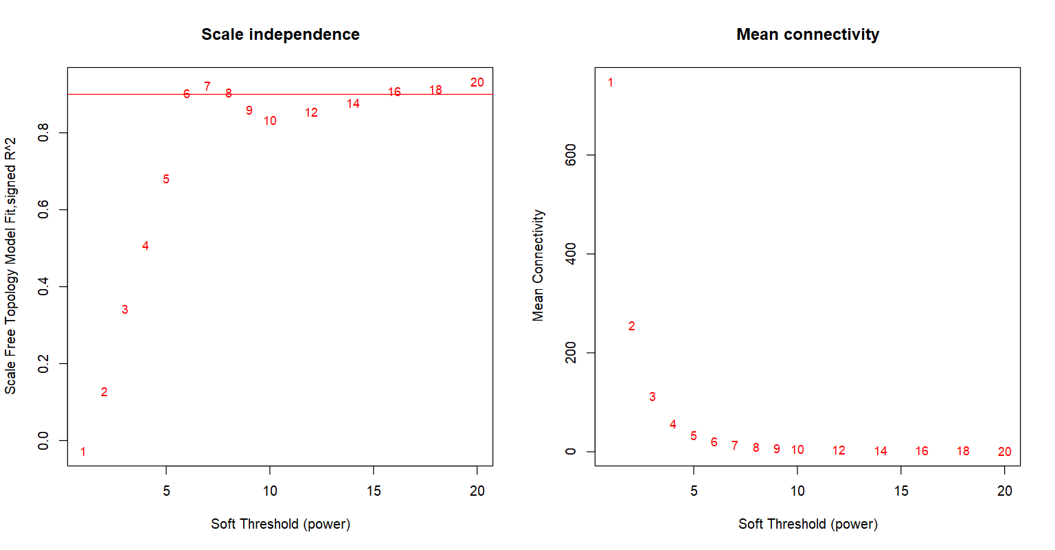
### （1）是否符合幂律分布；
plot(sft$fitIndices[,1], -sign(sft$fitIndices[,3])*sft$fitIndices[,2],
     xlab="Soft Threshold (power)",ylab="Scale Free Topology Model Fit,signed R^2",type="n",
     main = paste("Scale independence"));
text(sft$fitIndices[,1], -sign(sft$fitIndices[,3])*sft$fitIndices[,2],
     labels=powers,cex=cex1,col="red")
abline(h=0.90,col="red")
### （2）节点的平均连接度
plot(sft$fitIndices[,1], sft$fitIndices[,5],
     xlab="Soft Threshold (power)",ylab="Mean Connectivity", type="n",
     main = paste("Mean connectivity"))
text(sft$fitIndices[,1], sft$fitIndices[,5], labels=powers, cex=cex1,col="red")

par(mfrow = c(1,1))

如下图所示，基本在6时，拟合幂律分布的结果是比较好的；同时节点的凭据连通性也趋于稳定了。之后会使用这个参数建立网络。

2.3 建立网络，鉴定模块

方式一：逐步分析

 1
 2
 3
 4
 5
 6
 7
 8
 9
10
11
12
13
14
15
16
17
18
19
20
21
22
23
24
25
26
27
28
29
30
31
32
33
34
35
36
37
38
39
40
41
42
43
44
45
46


##(1) 根据选定的软阈值，得出邻接矩阵
adjacency = adjacency(exp_dat, power = 6)
adjacency[1:4,1:4]
#               F2_2         F2_3        F2_14        F2_15
# F2_2  1.000000e+00 2.669773e-02 8.679043e-07 0.0285218325
# F2_3  2.669773e-02 1.000000e+00 1.491148e-06 0.1223727405
# F2_14 8.679043e-07 1.491148e-06 1.000000e+00 0.0007245466
# F2_15 2.852183e-02 1.223727e-01 7.245466e-04 1.0000000000

##(2)转为TOM矩阵
TOM = TOMsimilarity(adjacency)
TOM[1:4,1:4]
#              [,1]         [,2]         [,3]        [,4]
# [1,] 1.0000000000 0.0443291435 0.0006062579 0.033303820
# [2,] 0.0443291435 1.0000000000 0.0005190759 0.068058832
# [3,] 0.0006062579 0.0005190759 1.0000000000 0.002154665
# [4,] 0.0333038199 0.0680588319 0.0021546653 1.000000000

##(3)进一步转为不相似性矩阵（距离矩阵）
dissTOM = 1-TOM
dissTOM[1:4,1:4]
#           [,1]      [,2]      [,3]      [,4]
# [1,] 0.0000000 0.9556709 0.9993937 0.9666962
# [2,] 0.9556709 0.0000000 0.9994809 0.9319412
# [3,] 0.9993937 0.9994809 0.0000000 0.9978453
# [4,] 0.9666962 0.9319412 0.9978453 0.0000000

##(4) 层次聚类hierarchical clustering
geneTree = hclust(as.dist(dissTOM), method = "average")
##(5) 动态切割树，鉴定模块
dynamicMods = cutreeDynamic(dendro = geneTree, distM = dissTOM,
                            deepSplit = 2, pamRespectsDendro = FALSE,
                            minClusterSize = 30)
# dynamicMods
# 0   1   2   3   4   5   6   7   8   9  10  11  12  13  14  15  16  17  18  19  20  21  22 
# 88 614 316 311 257 235 225 212 158 153 121 106 102 100  94  91  78  76  65  58  58  48  34
##如上表示切割为22个基因模块，其中模块0表示 unassigned genes

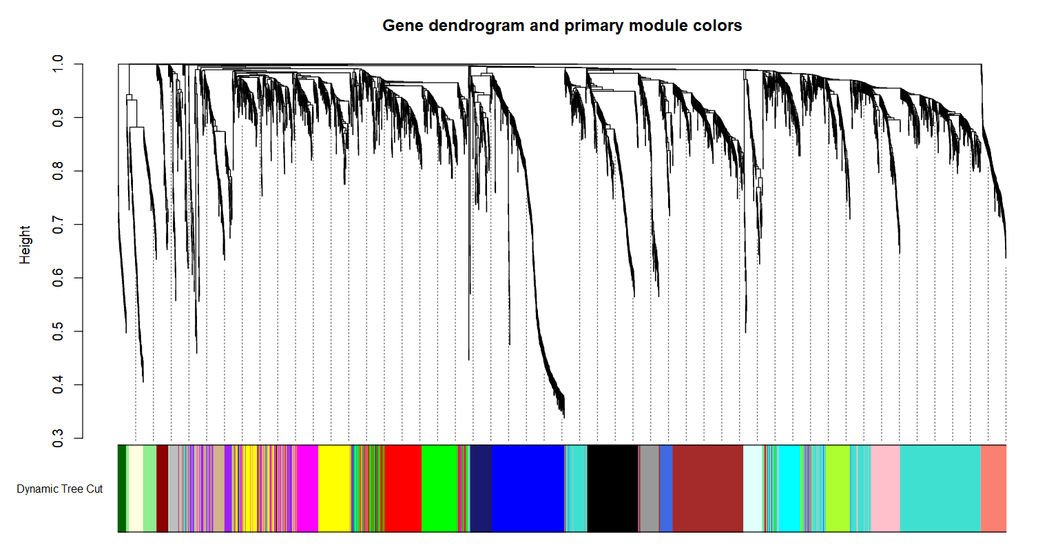
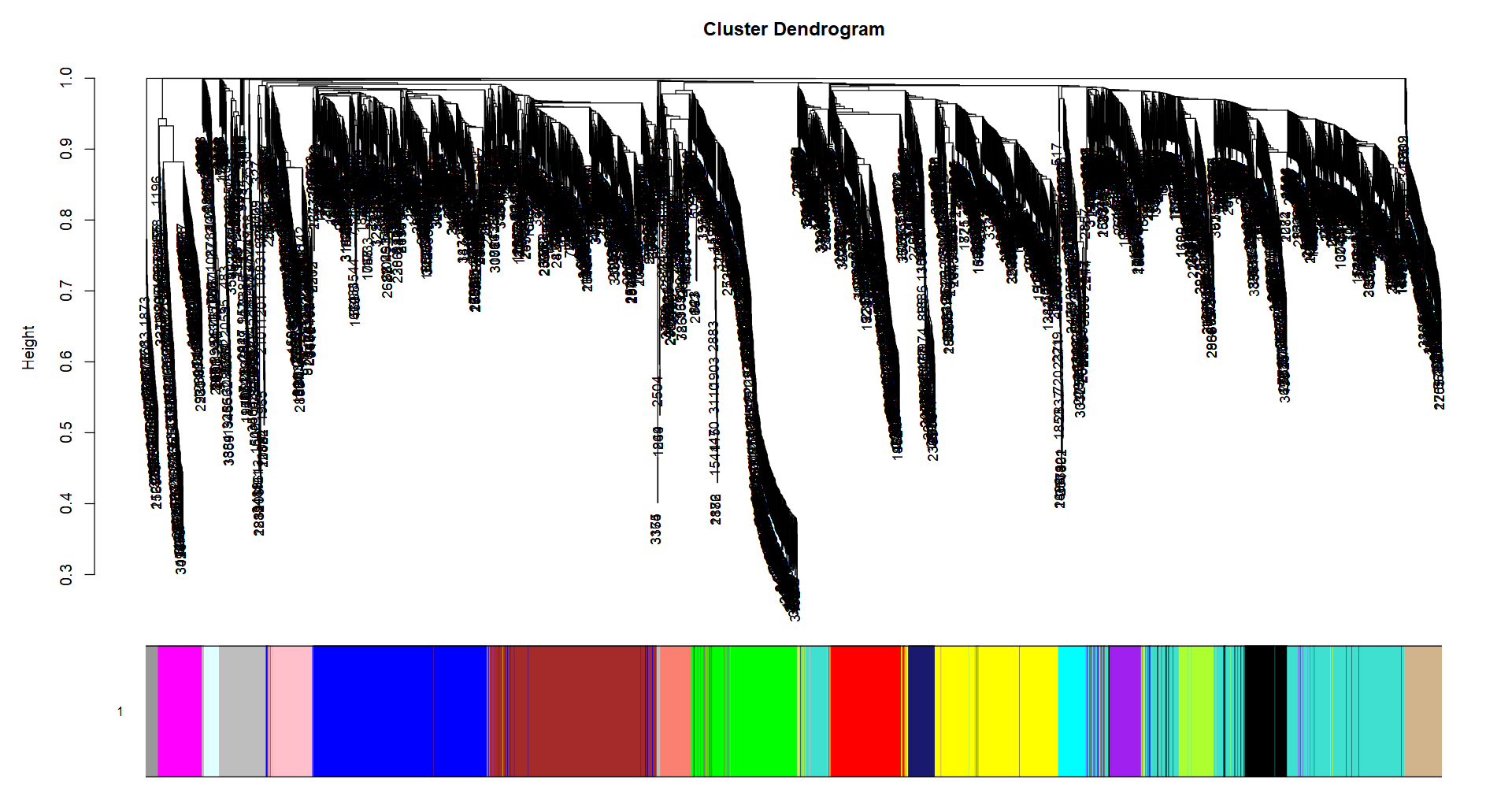
##(6)将模块名映射为颜色名，并可视化
dynamicColors = labels2colors(dynamicMods)
table(dynamicColors) #module0 会被映射到灰色 grey
sizeGrWindow(8,6)
plotDendroAndColors(geneTree, dynamicColors, "Dynamic Tree Cut",
                    dendroLabels = FALSE, hang = 0.03,
                    addGuide = TRUE, guideHang = 0.05,
                    main = "Gene dendrogram and primary module colors")

接下来需要判断有无非常相似的模块，进行合并操作

1
2
3
4
5
6
7
8
9


##(7)根据模块的特征值，计算不同模块的相似性，进行层次聚类
MEList = moduleEigengenes(exp_dat, colors = dynamicColors)
MEs = MEList$eigengenes
MEDiss = 1-cor(MEs)
METree = hclust(as.dist(MEDiss), method = "average")
sizeGrWindow(7, 6)
plot(METree, main = "Clustering of module eigengenes",
     xlab = "", sub = "")
abline(h=0.25, col = "red")  #根据实际情况而定

 1
 2
 3
 4
 5
 6
 7
 8
 9
10
11
12


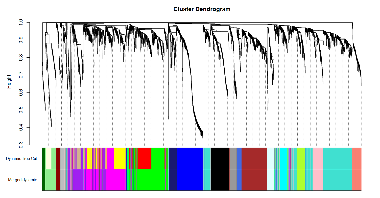
##(8)根据选择的阈值，合并模块
merge = mergeCloseModules(exp_dat, dynamicColors, cutHeight = 0.25)
#新划分模块的颜色映射
mergedColors = merge$colors
#新划分模块的特征值
mergedMEs = merge$newMEs
#可视化合并前后的模块
sizeGrWindow(12, 9)
plotDendroAndColors(geneTree, cbind(dynamicColors, mergedColors),
                    c("Dynamic Tree Cut", "Merged dynamic"),
                    dendroLabels = FALSE, hang = 0.03,
                    addGuide = TRUE, guideHang = 0.05)

方式二：一步分析

WGCNA包提供了blockwiseModules()函数可将上述步骤打包在一起，一次执行建立网络、鉴定模块的分析。

结合逐步分析，可以看到有一些关键参数可以调节：

power：软阈值的选择
corType：计算相关性的方法；可选pearson(默认)，bicor。后者更能考虑离群点的影响。
networkType:计算邻接矩阵时，是否考虑正负相关性；默认为"unsigned",可选"signed", “signed hybrid”
TOMType：计算TOM矩阵时，是否考虑正负相关性；默认为"signed",可选"unsigned"。但是根据幂律转换的邻接矩阵(权重)的非负性，所以认为这里选择"signed"也没有太多的意义。
minModuleSize：模块的最少基因数
mergeCutHeight：合并模块的阈值
numericLabels：模块名是否为数字；若设置FALSE，表示映射为颜色名。
saveTOMs：是否保存TOM矩阵；如果设为TRUE，需要设置saveTOMFileBase参数，提供保存文件名；设置numericLabels参数，是否将模块名保存为颜色名
nThreads ：交代线程数，适用于Linux环境
verbose：0默认安静的执行，值越大表示给出的运行提示信息越多。

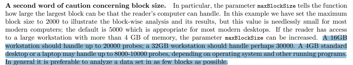
关于blocks相关参数：主要是考虑到输入基因数太大，电脑运行内存不足的情况。默认为"NULL"，即全部一次运行，不分多个blocks。

 1
 2
 3
 4
 5
 6
 7
 8
 9
10
11


net = blockwiseModules(exp_dat, power = 6,
                       corType = "pearson",
                       networkType="unsigned",
                       TOMType = "unsigned", 
                       minModuleSize = 30,
                       mergeCutHeight = 0.25,
                       verbose = 3)

names(net)
# [1] "colors"         "unmergedColors" "MEs"            "goodSamples"    "goodGenes"     
# [6] "dendrograms"    "TOMFiles"       "blockGenes"     "blocks"         "MEsOK"  

解析结果list结构

 1
 2
 3
 4
 5
 6
 7
 8
 9
10
11
12
13
14
15
16
17


#(1) 最终得到的网络模块(合并之后)
unique(net$colors)
table(net$colors)
# grey module是 unassigned gene

##合并之前的网络模块
unique(net$unmergedColors)
table(net$unmergedColors)

#(2) 134个样本对于18个模块的特征值
dim(net$MEs)
net$MEs[1:4,1:4]
net$MEsOK

#(3)聚类树状图，color注释模块
plotDendroAndColors(dendro = net$dendrograms[[1]],
                    colors = net$colors)

2.4 关联表型分析

以2.3 方式二得到结果继续分析

 1
 2
 3
 4
 5
 6
 7
 8
 9
10
11
12
13
14
15
16
17
18
19
20
21
22
23
24
25
26
27
28
29
30
31
32
33
34
35
36
37
38
39
40


# (1)计算模块特征值
# MEs = moduleEigengenes(exp_dat, net$colors)$eigengenes
MEs = net$MEs
MEs = orderMEs(MEs)

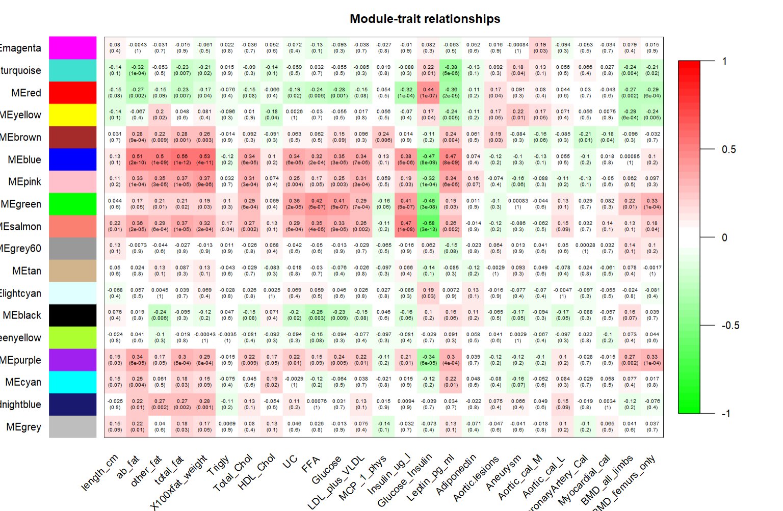
# (2)计算18个module与25个表型的相关性以及对应的P值
moduleTraitCor = cor(MEs, trait_dat, use = "p")
moduleTraitCor[1:4,1:4]
#               length_cm       ab_fat  other_fat   total_fat
# MEmagenta    0.08015682 -0.004282784 -0.0311292 -0.01504395
# MEturquoise -0.14101586 -0.323615446 -0.0528274 -0.23393609
# MEred       -0.15070061 -0.268348526 -0.1458333 -0.23102647
# MEyellow    -0.13732537 -0.067163777  0.1958153  0.04806599

moduleTraitPvalue = corPvalueStudent(moduleTraitCor, nrow(MEs))
moduleTraitPvalue[1:4,1:4]
#              length_cm       ab_fat  other_fat   total_fat
# MEmagenta   0.35722181 0.9608295943 0.72104901 0.863025117
# MEturquoise 0.10411666 0.0001366333 0.54437147 0.006518482
# MEred       0.08219621 0.0017187522 0.09269921 0.007237730
# MEyellow    0.11358818 0.4406688535 0.02336043 0.581283912

# (3)可视化相关性与P值
sizeGrWindow(10,6)
# Will display correlations and their p-values
textMatrix = paste(signif(moduleTraitCor, 2), "\n(",
                   signif(moduleTraitPvalue, 1), ")", sep = "")
dim(textMatrix) = dim(moduleTraitCor)
par(mar = c(6, 8.5, 3, 3))
labeledHeatmap(Matrix = moduleTraitCor,
               xLabels = names(trait_dat),
               yLabels = names(MEs),
               ySymbols = names(MEs),
               colorLabels = FALSE,
               colors = greenWhiteRed(50),
               textMatrix = textMatrix,
               setStdMargins = FALSE,
               cex.text = 0.5,
               zlim = c(-1,1),
               main = paste("Module-trait relationships"))

 1
 2
 3
 4
 5
 6
 7
 8
 9
10
11
12
13
14
15
16
17
18
19
20
21
22
23
24
25
26
27
28
29
30
31
32
33
34
35
36
37
38
39
40
41
42
43
44


##计算指定表型的相关分析
weight = trait_dat[,"X100xfat_weight",drop=F]
colnames(weight) = "weight"
# (1) Gene significance，GS：即比较样本某个基因与对应表型的相关性
GS_weight = as.data.frame(cor(exp_dat, weight, use = "p"))
colnames(GS_weight) = "GS_weight"
head(GS_weight)
#               GS_weight
# MMT00000044 -0.06788487
# MMT00000046 -0.09806093
# MMT00000051  0.20311624

GS.p_weight = as.data.frame(corPvalueStudent(as.matrix(GS_weight), nrow(exp_dat)))
#            GS.p_weight
# MMT00000044 0.43576664
# MMT00000046 0.25964873
# MMT00000051 0.01858241


# (2) Module Membership: 模块内基因表达与模块特征值的相关性
modNames = substring(names(MEs), 3)
# 计算3600个基因与18个模块的相关性
MM = as.data.frame(cor(exp_dat, MEs, use = "p"))
colnames(MM) = paste("MM", modNames, sep="")
MM[1:4,1:4]

MMPvalue = as.data.frame(corPvalueStudent(as.matrix(MM), nrow(exp_dat)))
MMPvalue = as.data.frame(corPvalueStudent(as.matrix(MM), nrow(exp_dat)));
colnames(MMPvalue) = paste("p.MM", modNames, sep="");
MMPvalue[1:4,1:4]

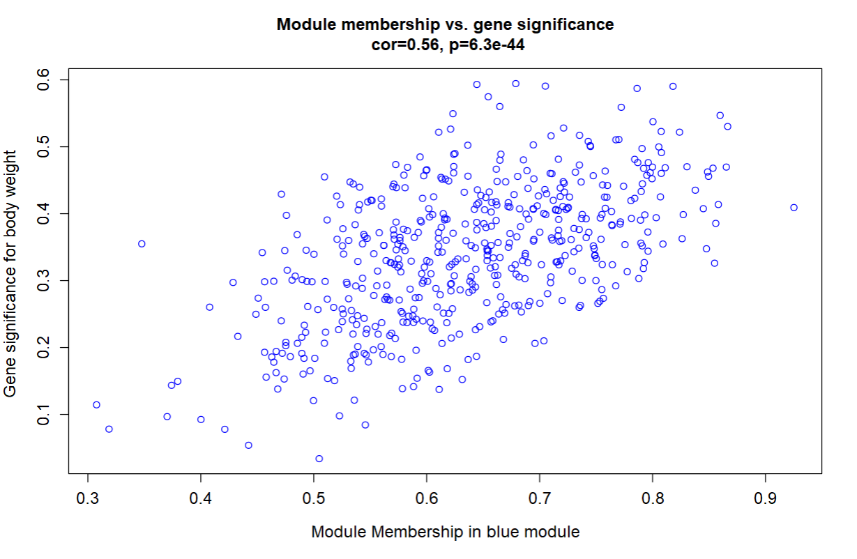
# (3) 可视化blue模块基因特征
# identical(rownames(MM), names(net$colors))
# TRUE
module = "blue"
moduleGenes = names(net$colors)[net$colors=="blue"]
sizeGrWindow(7, 7)
par(mfrow = c(1,1))
verboseScatterplot(abs(MM[moduleGenes, "MMblue"]),
                   abs(GS_weight[moduleGenes, 1]),
                   xlab = paste("Module Membership in", module, "module"),
                   ylab = "Gene significance for body weight",
                   main = paste("Module membership vs. gene significance\n"),
                   cex.main = 1.2, cex.lab = 1.2, cex.axis = 1.2, col = module)

可视化blue模块内的基因特征。当基因与blue模块越相关时，该基因也与该表型Trait相关。

2.5 挑选模块Hub基因

关于模块的Hub基因，WGCNA并没有明确的筛选方法。

 1
 2
 3
 4
 5
 6
 7
 8
 9
10
11
12
13
14
15
16
17
18
19
20
21
22
23
24
25
26
27


## (1) 模块内基因连接度
adjacency = adjacency(exp_dat, power = 6)
# TOM = TOMsimilarity(adjacency)
TOM[1:4,1:4]
Alldegrees =intramodularConnectivity(adjacency, net$colors)
head(Alldegrees)
#                 kTotal    kWithin       kOut      kDiff
# MMT00000044  0.4092743  0.2862358  0.1230385  0.1631973
# MMT00000046 37.8927830 24.9652317 12.9275513 12.0376805
# MMT00000051 28.3866248 17.2076759 11.1789488  6.0287271
# MMT00000076  1.3015473  1.1992420  0.1023053  1.0969366
# MMT00000080 25.9713107 16.3954194  9.5758914  6.8195280
# MMT00000102 10.5051504  2.4713718  8.0337786 -5.5624067

#### kTotal:基因在整个网络中的连接度
#### kWithin: 基因在所属模块中的连接度，即Intramodular connectivity
#### kOut: kTotal-kWithin
#### kDiff: kIn-kOut

#也可以绘制一个模块基因的Intramodular connectivity与Gene significance的散点图


## (2) Module Membership: 即上一节计算的模块内基因表达与模块特征值的相关性。

## (3) Gene significance，GS：即比较样本某个基因与对应表型的相关性

## (4) 综合上述指标，自定义合适阈值，选取一定数量的模块Hub基因。

1、关于WGCNA原理#

1.1 建立共表达网络#

（1）similarity matrix#

（2）adjacency matrix#

（3）topological overlap matrix#

1.2 鉴定模块及相关分析#

2、WGCNA实操#

2.1 整理输入数据#

2.2 选择合适的软阈值β#

2.3 建立网络，鉴定模块#

方式一：逐步分析#

方式二：一步分析#

2.4 关联表型分析#

2.5 挑选模块Hub基因#