TCGAbiolinks包是一站式分析TCGA数据的R包工具，它集成了TCGA数据下载、分析、可视化的全部流程。此次系列笔记主要跟着 TCGAbiolinks帮助文档重新学习下TCGA数据挖掘流程。

官方文档：https://bioconductor.org/packages/release/bioc/vignettes/TCGAbiolinks/inst/doc/index.html

文献：TCGAbiolinks: an R/Bioconductor package for integrative analysis of TCGA data https://pubmed.ncbi.nlm.nih.gov/26704973/
安装包
1
2
3
4
5
6
7
if (!requireNamespace("BiocManager", quietly = TRUE))
    install.packages("BiocManager")
#From github
BiocManager::install("BioinformaticsFMRP/TCGAbiolinksGUI.data")
BiocManager::install("BioinformaticsFMRP/TCGAbiolinks")
#From Bioconductor
BiocManager::install("TCGAbiolinks")

一、查找TCGA数据

主要通过GDCquery()函数查找数据

 1
 2
 3
 4
 5
 6
 7
 8
 9
10
11
12
13
14
15


library(TCGAbiolinks)
GDCquery(
  project,
  data.category,
  data.type,
  workflow.type,
  legacy = FALSE,
  access,
  platform,
  file.type,
  barcode,
  data.format,
  experimental.strategy,
  sample.type
)

1 选择肿瘤类型

project参数：指定一个或多个感兴趣的TCGA项目名
如下代码所示，供包括33种TCGA癌症类型。癌症简称对应全称及中文名见文末。

1
2
3
4
5
6
7
8
9


projects = TCGAbiolinks:::getGDCprojects()$project_id
TCGAs = grep("TCGA", projects, value = T)
sort(TCGAs)
# [1] "TCGA-ACC"  "TCGA-BLCA" "TCGA-BRCA" "TCGA-CESC" "TCGA-CHOL" "TCGA-COAD"
# [7] "TCGA-DLBC" "TCGA-ESCA" "TCGA-GBM"  "TCGA-HNSC" "TCGA-KICH" "TCGA-KIRC"
# [13] "TCGA-KIRP" "TCGA-LAML" "TCGA-LGG"  "TCGA-LIHC" "TCGA-LUAD" "TCGA-LUSC"
# [19] "TCGA-MESO" "TCGA-OV"   "TCGA-PAAD" "TCGA-PCPG" "TCGA-PRAD" "TCGA-READ"
# [25] "TCGA-SARC" "TCGA-SKCM" "TCGA-STAD" "TCGA-TGCT" "TCGA-THCA" "TCGA-THYM"
# [31] "TCGA-UCEC" "TCGA-UCS"  "TCGA-UVM" 

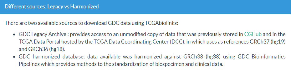
2 hg19/hg38

主要根据参考基因组的不同，包含两套数据：GDC Legacy Archive【主要GRCh37 (hg19)】，GDC harmonized database【GRCh38 (hg38)】
通过设置参数legacy ，默认为FALSE(hg38)；TRUE则表示使用hg19参考基因组的测序数据。

3 下载数据类型

基于上述的参数，我们可以设置如下参数，交代我们的目标数据类型

data.category = 指定下载什么类型的数据：如转录组数据、临床数据….

 1
 2
 3
 4
 5
 6
 7
 8
 9
10
11
12
13
14
15


##(1) GDC harmonized database【GRCh38 (hg38)】
TCGAbiolinks:::getProjectSummary("TCGA-BRCA", legacy = FALSE)$data_categories$data_category
# [1] "Structural Variation"        "Simple Nucleotide Variation"
# [3] "Copy Number Variation"       "Transcriptome Profiling"    
# [5] "DNA Methylation"             "Sequencing Reads"           
# [7] "Biospecimen"                 "Clinical"                   
# [9] "Proteome Profiling"  

##(2) GDC Legacy Archive【主要GRCh37 (hg19)】
TCGAbiolinks:::getProjectSummary("TCGA-BRCA", legacy = TRUE)$data_categories$data_category
# [1] "Protein expression"          "Copy number variation"      
# [3] "Biospecimen"                 "Simple nucleotide variation"
# [5] "Gene expression"             "Raw microarray data"        
# [7] "DNA methylation"             "Clinical"                   
# [9] "Raw sequencing data"

data.type = 更加细节的数据类型选择，例如harmonized的Transcriptome Profiling有 Gene Expression Quantification, Isoform Expression Quantification, miRNA Expression Quantification, Splice Junction Quantification4种数据。而我们一般需要的是Gene Expression Quantification。
workflow.type = 同一个测序数据可能有不同的pipeline处理流程，如果有不同的处理流程，需要选择。据最新的TCGA版本，仅提供STAR - Counts。
platform = 测序平台（optional）
file.type = 具体的数据文件（optional, for legacy）如果不知道目标数据的上述信息，可以参考下面的概述

具体参考文末第二点。

4 样本标签Barcode

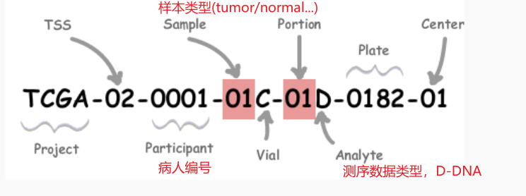
完整的barcode：形如 TCGA-G4-6317-02A-11D-2064-05，这个标签包含了从病人来源到测序过程、分析的所有信息，如下图所示比较重要的是Participant、Sample 、Portion三个部分，分别交代了病人编号、样本类型、测序类型病人的id：形如 TCGA-G4-6317 样本来源的id：形如 TCGA-G4-6317-02

其中比较重要的是交代样本类型的Sample的两位数信息，是后面进行差异分析的分组依据。具体对应的含义如下。例如01表示病人的原位瘤组织；11表示来自病人的正常组织….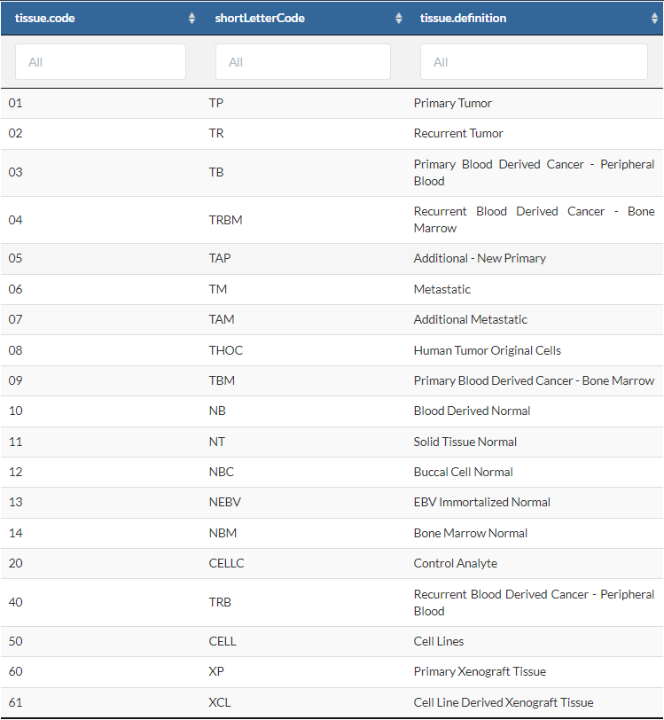
基于上述理解，我们也可以设置sample.type = 参数指定下载感兴趣的样本类型数据，例如sample.type = "Primary Tumor"
对于给定的TCGA barcode，可以利用TCGAquery_SampleTypes()提取出目标分组的样本；TCGAquery_MatchedCoupledSampleTypes()函数可以提取来自同一病人的配对样本数据。

 1
 2
 3
 4
 5
 6
 7
 8
 9
10
11
12
13
14
15
16
17
18
19
20
21
22
23
24
25
26
27
28


query <- GDCquery(project = c("TCGA-BRCA"),
                  legacy = FALSE, 
                  data.category = "Transcriptome Profiling",
                  data.type = "Gene Expression Quantification",
                  workflow.type = "HTSeq - Counts")
dim(getResults(query))
#[1] 1222   29
query_info = getResults(query)
TP = TCGAquery_SampleTypes(query_info$sample.submitter_id,"TP")
NT = TCGAquery_SampleTypes(query_info$sample.submitter_id,"NT")
query <- GDCquery(project = c("TCGA-BRCA"),
                  legacy = FALSE, 
                  data.category = "Transcriptome Profiling",
                  data.type = "Gene Expression Quantification",
                  workflow.type = "HTSeq - Counts",
                  barcode = c(TP, NT))
dim(getResults(query))
#[1] 1215   29

Pair_sample = TCGAquery_MatchedCoupledSampleTypes(query_info$sample.submitter_id,c("NT","TP"))
query <- GDCquery(project = c("TCGA-BRCA"),
                  legacy = FALSE, 
                  data.category = "Transcriptome Profiling",
                  data.type = "Gene Expression Quantification",
                  workflow.type = "HTSeq - Counts",
                  barcode = Pair_sample)
dim(getResults(query))
#[1] 229  29

如上是查询TCGA目标数据的几种常见标准，还有几个参数没有介绍，可参看函数帮助文档。可根据自己的目的灵活设置上述参数。

二、从数据下载到差异分析

以胆管癌为例，演示从数据下载到差异分析的全流程。

1 Legacy(hg19)

1.1 下载数据

 1
 2
 3
 4
 5
 6
 7
 8
 9
10
11
12
13
14
15


library(TCGAbiolinks)
##(1) 获取下载目标文件
query <- GDCquery(project = "TCGA-CHOL",
                  legacy = TRUE,
                  data.category = "Gene expression",
                  data.type = "Gene expression quantification",
                  platform = "Illumina HiSeq", 
                  file.type  = "results")

##(2) 下载数据到本地
# files.per.chunk = 10 表示分批下载，每批下载10个病人的数据，可避免中途报错，而前功尽弃。
GDCdownload(query, files.per.chunk = 10)

##(3) 加载数据至当前环境
data <- GDCprepare(query, save = T, save.filename = "CHOL_RNAseq_hg19.rda")

1.2 探索数据

 1
 2
 3
 4
 5
 6
 7
 8
 9
10
11
12
13
14
15
16
17
18
19
20
21
22
23
24
25
26
27


library(SummarizedExperiment)
dim(assay(data))
#[1] 19947    45

##(1) 查看表达矩阵
assayNames(data)
# [1] "raw_count"       "scaled_estimate"
assay(data, "raw_count")[1:3,1:3]
#        TCGA-W5-AA2I-11A-11R-A41I-07 TCGA-W5-AA2U-11A-11R-A41I-07 TCGA-W5-AA2I-01A-32R-A41I-07
# A1BG|1                     80062.65                      79948.1                      2519.20
# A2M|2                      79697.45                     126813.9                      4107.88
# NAT1|9                       364.00                        397.0                       126.00

##(2) 样本(临床)信息
dim(colData(data))
#[1]  45 201
colData(data)[1:4,1:4]

##(3) 基因信息
rowData(data)[1:6,1:5]
# DataFrame with 6 rows and 3 columns
#                   gene_id entrezgene ensembl_gene_id
#                   <character>  <integer>     <character>
# A1BG                 A1BG          1 ENSG00000121410
# A2M                   A2M          2 ENSG00000175899
# NAT1                 NAT1          9 ENSG00000171428
rowRanges(data)

1.3 整理数据

 1
 2
 3
 4
 5
 6
 7
 8
 9
10
11
12
13
14
15
16
17
18
19
20
21
22
23
24
25
26
27
28
29
30
31
32
33
34
35


##(1)更改表达矩阵行名/基因名格式
rownames(data) = stringr::str_split(rownames(data),
                                    "[|]", simplify = T)[,1]
data = data[!duplicated(rownames(data)),]
dim(data)
# [1] 19938    45
assay(data, "raw_count")[1:3,1:3]
#        TCGA-W5-AA2I-11A-11R-A41I-07 TCGA-W5-AA2U-11A-11R-A41I-07 TCGA-W5-AA2I-01A-32R-A41I-07
# A1BG                     80062.65                      79948.1                      2519.20
# A2M                      79697.45                     126813.9                      4107.88
# NAT1                       364.00                        397.0                       126.00


##(2) 分析样本间相关性，鉴定离群点样本
CorOutliers <- TCGAanalyze_Preprocessing(data, cor.cut = 0, 
                                         filename="CHOL45_hg19_cor.png")

##(3) 标准化
dataNorm <- TCGAanalyze_Normalization(tabDF = data, geneInfo =  geneInfo) #没有log处理
dim(dataNorm)
# [1] 17618    45
class(dataNorm) 
# [1] "matrix" "array"
dataNorm[1:3,1:3]
#      TCGA-W5-AA2I-11A-11R-A41I-07 TCGA-W5-AA2U-11A-11R-A41I-07 TCGA-W5-AA2I-01A-32R-A41I-07
# A1BG                        80063                        79948                         2519
# A2M                         79697                       126814                         4108
# NAT1                          364                          397                          126

##(4) 过滤低表达基因
dataFilt <- TCGAanalyze_Filtering(tabDF = dataNorm,
                                  method = "quantile", 
                                  qnt.cut =  0.05)
dim(dataFilt)
exp_data = dataFilt

1.4 差异分析

 1
 2
 3
 4
 5
 6
 7
 8
 9
10
11
12
13
14
15
16
17
18
19
20
21
22
23
24
25
26
27
28
29
30
31
32
33


##(1) 确定分组样本
samplesNT <- TCGAquery_SampleTypes(barcode = colnames(exp_data),
                                   typesample = c("NT"))
samplesTP <- TCGAquery_SampleTypes(barcode = colnames(exp_data), 
                                   typesample = c("TP"))

##(2) 差异分析
dataDEGs <- TCGAanalyze_DEA(mat1 = exp_data[,samplesNT],
                            mat2 = exp_data[,samplesTP],
                            Cond1type = "Normal",
                            Cond2type = "Tumor",
                            pipeline = "edgeR",
                            method = "glmLRT")
##(3) 整理结果
DEGs <- TCGAanalyze_LevelTab(dataDEGs,"Tumor","Normal",
                             exp_data[,samplesTP],exp_data[,samplesNT])
DEGs = DEGs[order(DEGs$FDR),]
DEGs$Direct = ifelse(DEGs$logFC>0, "Up", "Down")
head(DEGs)
#          mRNA     logFC          FDR      Delta      Tumor      Normal Direct
# USH2A   USH2A -5.261122 1.805847e-46  -150.9650   28.69444  1207.88889   Down
# KCNN2   KCNN2 -4.344681 1.045519e-36  -188.2695   43.33333   893.77778   Down
# LCAT     LCAT -3.683368 2.344098e-31 -1875.2437  509.11111  6640.22222   Down
# IQCE     IQCE  4.229960 6.301169e-30 12462.2846 2946.19444   153.33333     Up
# DCXR     DCXR -4.070648 9.023484e-30 -7408.0132 1819.86111 32284.22222   Down
# PRSS16 PRSS16  6.947385 3.517876e-28  9163.9866 1319.05556    10.22222     Up

DEGs = DEGs[order(DEGs$FDR),]
DEGs$Direct = ifelse(DEGs$logFC>0, "Up", "Down")
table(DEGs$FDR<0.01,DEGs$Direct)

DEGs_sig = subset(DEGs, FDR<0.01)
table(DEGs_sig$Direct, abs(DEGs_sig$logFC)>1)

2 Harmonized(hg38)

2.1 下载数据

 1
 2
 3
 4
 5
 6
 7
 8
 9
10
11
12
13


library(TCGAbiolinks)
##(1) 获取下载目标文件
query <- GDCquery(project = "TCGA-CHOL",
                  legacy = FALSE,
                  data.category = "Transcriptome Profiling",
                  data.type = "Gene Expression Quantification")

##(2) 下载数据到本地
# files.per.chunk = 10 表示分批下载，每批下载10个病人的数据，可避免中途报错，而前功尽弃。
GDCdownload(query, files.per.chunk = 10)

##(3) 加载数据至当前环境
data <- GDCprepare(query, save = T, save.filename = "CHOL_RNAseq_hg38.rda")

2.2 探索数据

 1
 2
 3
 4
 5
 6
 7
 8
 9
10
11
12
13
14
15
16
17
18
19
20
21
22
23
24
25
26
27
28
29
30
31
32
33
34
35
36
37


library(SummarizedExperiment)
dim(assay(data))
#[1] 60660    44

##(1) 查看表达矩阵
assayNames(data)
#[1] "unstranded"       "stranded_first"   "stranded_second"  "tpm_unstrand"    
#[5] "fpkm_unstrand"    "fpkm_uq_unstrand"
assay(data, "unstranded")[1:3,1:3]
#                    TCGA-W5-AA2X-01A-11R-A41I-07 TCGA-W5-AA2X-11A-11R-A41I-07 TCGA-W5-AA33-01A-11R-A41I-07
# ENSG00000000003.15                         3310                         2322                        11312
# ENSG00000000005.6                             0                            0                            1
# ENSG00000000419.13                         1881                          716                          968

##(2) 样本(临床)信息
dim(colData(data))
#[1]  44 201
colData(data)[1:4,1:4]

##(3) 基因信息
t(rowData(data)[1,])
# TransposedDataFrame with 10 rows and 1 column
#                           ENSG00000000003.15
# source      <factor>                  HAVANA
# type        <factor>                    gene
# score       <numeric>                     NA
# phase       <integer>                     NA
# gene_id     <character>   ENSG00000000003.15
# gene_type   <character>       protein_coding
# gene_name   <character>               TSPAN6
# level       <character>                    2
# hgnc_id     <character>           HGNC:11858
# havana_gene <character> OTTHUMG00000022002.2
table(rowData(data)$gene_type) %>% sort(decreasing = T)  %>% head()
# protein_coding                 lncRNA   processed_pseudogene unprocessed_pseudogene               misc_RNA                  snRNA 
#          19962                  16901                  10167                   2614                   2212                   1901 
rowRanges(data)

2.3 整理数据

 1
 2
 3
 4
 5
 6
 7
 8
 9
10
11
12
13
14
15
16
17
18
19
20
21
22
23
24
25
26
27
28
29
30
31
32
33
34
35


##(1)更改表达矩阵行名/基因名格式，筛选基因
rownames(data) = rowData(data)$gene_name
data = data[!duplicated(rownames(data)),]
data = data[rowData(data)$gene_type=="protein_coding",]
dim(data)
# [1] 19934    44
assay(data, "unstranded")[1:3,1:3]
#        TCGA-W5-AA2X-01A-11R-A41I-07 TCGA-W5-AA2X-11A-11R-A41I-07 TCGA-W5-AA33-01A-11R-A41I-07
# TSPAN6                         3310                         2322                        11312
# TNMD                              0                            0                            1
# DPM1                           1881                          716                          968


##(2) 分析样本间相关性，鉴定离群点样本
CorOutliers <- TCGAanalyze_Preprocessing(data, cor.cut = 0, 
                                         filename="CHOL45_hg38_cor.png")

##(3) 标准化
dataNorm <- TCGAanalyze_Normalization(tabDF = data, geneInfo =  geneInfo) #没有log处理
dim(dataNorm)
# [1] 15196    44
class(dataNorm) 
# [1] "matrix" "array"
dataNorm[1:3,1:3]
#        TCGA-W5-AA2X-01A-11R-A41I-07 TCGA-W5-AA2X-11A-11R-A41I-07 TCGA-W5-AA33-01A-11R-A41I-07
# TSPAN6                         3310                         2322                        11312
# DPM1                           1881                          716                          968
# SCYL3                           966                          315                         1296

##(4) 过滤低表达基因
# dataFilt <- TCGAanalyze_Filtering(tabDF = dataNorm,
#                                   method = "quantile", 
#                                   qnt.cut =  0.05)
# dim(dataFilt)
exp_data = dataNorm

2.4 差异分析

(1) edgeR

 1
 2
 3
 4
 5
 6
 7
 8
 9
10
11
12
13
14
15
16
17
18
19
20
21
22
23
24
25
26
27
28
29
30
31
32
33


##(1) 确定分组样本
samplesNT <- TCGAquery_SampleTypes(barcode = colnames(exp_data),
                                   typesample = c("NT"))
samplesTP <- TCGAquery_SampleTypes(barcode = colnames(exp_data), 
                                   typesample = c("TP"))

##(2) 差异分析
dataDEGs <- TCGAanalyze_DEA(mat1 = exp_data[,samplesNT],
                            mat2 = exp_data[,samplesTP],
                            Cond1type = "Normal",
                            Cond2type = "Tumor",
                            pipeline = "edgeR",
                            method = "glmLRT")
##(3) 整理结果
DEGs <- TCGAanalyze_LevelTab(dataDEGs,"Tumor","Normal",
                             exp_data[,samplesTP],exp_data[,samplesNT])
DEGs = DEGs[order(DEGs$FDR),]
DEGs$Direct = ifelse(DEGs$logFC>0, "Up", "Down")
head(DEGs)
#          mRNA     logFC          FDR      Delta      Tumor      Normal Direct
# USH2A   USH2A -5.261122 1.805847e-46  -150.9650   28.69444  1207.88889   Down
# KCNN2   KCNN2 -4.344681 1.045519e-36  -188.2695   43.33333   893.77778   Down
# LCAT     LCAT -3.683368 2.344098e-31 -1875.2437  509.11111  6640.22222   Down
# IQCE     IQCE  4.229960 6.301169e-30 12462.2846 2946.19444   153.33333     Up
# DCXR     DCXR -4.070648 9.023484e-30 -7408.0132 1819.86111 32284.22222   Down
# PRSS16 PRSS16  6.947385 3.517876e-28  9163.9866 1319.05556    10.22222     Up

DEGs = DEGs[order(DEGs$FDR),]
DEGs$Direct = ifelse(DEGs$logFC>0, "Up", "Down")
table(DEGs$FDR<0.01,DEGs$Direct)

DEGs_sig = subset(DEGs, FDR<0.01)
table(DEGs_sig$Direct, abs(DEGs_sig$logFC)>1)

(2) Deseq2

 1
 2
 3
 4
 5
 6
 7
 8
 9
10
11
12
13
14
15
16
17
18
19
20
21
22
23
24
25
26
27
28
29
30
31
32
33
34
35
36
37
38
39
40
41
42
43
44
45
46


##(1)Deseq2差异分析
library(TCGAbiolinks)
library(DESeq2)
library(tidyverse)
data$sample_type = factor(data$sample_type, 
                          levels = c("Solid Tissue Normal","Primary Tumor"))
ddsSE <- DESeqDataSet(data, design = ~ sample_type)
keep <- rowSums(counts(ddsSE)) >= 10
ddsSE <- ddsSE[keep,]
ddsSE <- DESeq(ddsSE)
resultsNames(ddsSE)
res <- results(ddsSE, name = "sample_type_Primary.Tumor_vs_Solid.Tissue.Normal")
dea <- as.data.frame(res) %>% arrange(padj)
head(dea)
#        baseMean log2FoldChange     lfcSE      stat       pvalue         padj
# MSMO1 7585.3117      -3.748458 0.2108963 -17.77394 1.125105e-70 1.012094e-66
# RMDN2  396.7564      -2.929007 0.1648043 -17.77264 1.151350e-70 1.012094e-66
# GCDH  2272.8992      -3.302565 0.1863391 -17.72342 2.765888e-70 1.620903e-66
# TCAIM 1239.0498      -2.235399 0.1303361 -17.15104 6.174288e-66 2.713754e-62
# KCNN2  360.4370      -5.504733 0.3234314 -17.01979 5.858475e-65 2.059957e-61
# RCL1  2371.8288      -3.917907 0.2368974 -16.53842 1.940540e-61 5.686107e-58

##(2)配对差异分析
data_pair = data[,data$barcode  %in% TCGAquery_MatchedCoupledSampleTypes(data$barcode, c("NT","TP"))]
dim(data_pair)
data_pair$pair = substr(data_pair$barcode, 1, 12)
table(data_pair$pair)
# TCGA-W5-AA2I TCGA-W5-AA2Q TCGA-W5-AA2U TCGA-W5-AA2X TCGA-W5-AA30 TCGA-W5-AA31 TCGA-W5-AA34 TCGA-ZU-A8S4 
#            2            2            2            2            2            2            2            2
data_pair$sample_type = factor(data_pair$sample_type, 
                          levels = c("Solid Tissue Normal","Primary Tumor"))
ddsSE <- DESeqDataSet(data_pair, design = ~ sample_type + pair)
keep <- rowSums(counts(ddsSE)) >= 10
ddsSE <- ddsSE[keep,]
ddsSE <- DESeq(ddsSE)
resultsNames(ddsSE)
res <- results(ddsSE, name = "sample_type_Primary.Tumor_vs_Solid.Tissue.Normal")
dea_p <- as.data.frame(res) %>% arrange(padj)
head(dea_p)
#        baseMean log2FoldChange     lfcSE      stat        pvalue          padj
# PCK2  22698.702      -5.653596 0.1854224 -30.49037 3.496861e-204 5.903052e-200
# GRHPR 17379.001      -3.574709 0.1552370 -23.02743 2.476640e-117 2.090408e-113
# KDM8   1614.739      -4.555841 0.1989383 -22.90077 4.564515e-116 2.568453e-112
# CTH    2367.036      -5.254399 0.2324287 -22.60650 3.740448e-113 1.578563e-109
# ADI1  18162.322      -3.714172 0.1659180 -22.38559 5.438272e-111 1.836069e-107
# PBLD   8315.323      -5.683141 0.2593493 -21.91308 1.949637e-106 5.485303e-103

四、关于病人的临床数据与肿瘤分型

1、获取病人的临床数据

如上在GDCprepare()过程中，会自动注释病人样本的临床信息。
我们也可以预先单独下载每个病人的临床数据，以供参考。

方法一：GDCquery() pipeline

 1
 2
 3
 4
 5
 6
 7
 8
 9
10
11
12
13
14
15
16
17
18
19
20
21


query <- GDCquery(project = "TCGA-ACC", 
                  data.category = "Clinical",
                  data.type = "Clinical Supplement", 
                  data.format = "BCR Biotab")
GDCdownload(query, files.per.chunk = 20)
clinical.BCRtab.all <- GDCprepare(query)


grep("clinical_", names(clinical.BCRtab.all), value = T)
# [1] "clinical_drug_brca"               "clinical_omf_v4.0_brca"          
# [3] "clinical_follow_up_v4.0_brca"     "clinical_follow_up_v1.5_brca"    
# [5] "clinical_follow_up_v4.0_nte_brca" "clinical_patient_brca"           
# [7] "clinical_radiation_brca"          "clinical_nte_brca"               
# [9] "clinical_follow_up_v2.1_brca" 
clinical_patient_brca = as.data.frame(clinical.BCRtab.all$clinical_patient_brca)
clinical_patient_brca[1:4,1:4]
#                       bcr_patient_uuid bcr_patient_barcode form_completion_date                  prospective_collection
# 1                     bcr_patient_uuid bcr_patient_barcode form_completion_date tissue_prospective_collection_indicator
# 2                              CDE_ID:      CDE_ID:2003301              CDE_ID:                          CDE_ID:3088492
# 3 6E7D5EC6-A469-467C-B748-237353C23416        TCGA-3C-AAAU            2014-1-13                                      NO
# 4 55262FCB-1B01-4480-B322-36570430C917        TCGA-3C-AALI            2014-7-28                                      NO

方法二：GDCquery_clinic()

根据官方介绍，这个函数下载的是indexed clinical: a refined clinical data that is created using the XML files(方法一).
这种方法下载速度较快，建议优先使用。如果没有想要的信息，再使用方法一。

1
2
3
4
5
6
7
8


clinical <- GDCquery_clinic(project = "TCGA-BRCA", type = "clinical")
clinical <- GDCquery_clinic(project = "TCGA-BRCA", type = "clinical")
clinical[1:4,1:4]
#   submitter_id synchronous_malignancy ajcc_pathologic_stage tumor_stage
# 1 TCGA-E2-A14U                     No               Stage I     stage i
# 2 TCGA-E9-A1RC                     No            Stage IIIC  stage iiic
# 3 TCGA-D8-A1J9                     No              Stage IA    stage ia
# 4 TCGA-E2-A14P                     No            Stage IIIC  stage iiic

2、获取病人的肿瘤分型

PanCancerAtlas_subtypes() The columns “Subtype_Selected” was selected as most prominent subtype classification (from the other columns)

 1
 2
 3
 4
 5
 6
 7
 8
 9
10
11
12
13
14
15
16


subtypes <- PanCancerAtlas_subtypes()
dim(subtypes)
#[1] 7734   10
table(subtypes$cancer.type)
# ACC  AML BLCA BRCA COAD ESCA  GBM HNSC KICH KIRC KIRP  LGG LIHC LUAD LUSC OVCA PCPG 
# 91  187  129 1218  341  169  606  279   66  442  161  516  196  230  178  489  178 
# PRAD READ SKCM STAD THCA UCEC  UCS 
# 333  118  333  383  496  538   57
head(as.data.frame(subtypes))
#   pan.samplesID cancer.type                         Subtype_mRNA   Subtype_DNAmeth Subtype_protein Subtype_miRNA Subtype_CNA Subtype_Integrative Subtype_other      Subtype_Selected
# 1  TCGA-OR-A5J1         ACC steroid-phenotype-high+proliferation         CIMP-high              NA       miRNA_1       Quiet                COC3           C1A         ACC.CIMP-high
# 2  TCGA-OR-A5J2         ACC steroid-phenotype-high+proliferation          CIMP-low               1       miRNA_1       Noisy                COC3           C1A          ACC.CIMP-low
# 3  TCGA-OR-A5J3         ACC               steroid-phenotype-high CIMP-intermediate               3       miRNA_6 Chromosomal                COC2           C1A ACC.CIMP-intermediate
# 4  TCGA-OR-A5J4         ACC                                 <NA>         CIMP-high              NA       miRNA_6 Chromosomal                <NA>          <NA>         ACC.CIMP-high
# 5  TCGA-OR-A5J5         ACC               steroid-phenotype-high CIMP-intermediate              NA       miRNA_2 Chromosomal                COC2           C1A ACC.CIMP-intermediate
# 6  TCGA-OR-A5J6         ACC                steroid-phenotype-low          CIMP-low               2       miRNA_1       Noisy                COC1           C1B          ACC.CIMP-low

TCGAquery_subtype() These subtypes will be automatically added in the summarizedExperiment object through GDCprepare. But you can also use the TCGAquery_subtype function to retrieve this information.

 1
 2
 3
 4
 5
 6
 7
 8
 9
10
11
12
13
14
15
16
17
18
19
20
21
22
23
24
25
26
27


brca.subtype <- TCGAquery_subtype(tumor = "brca")
t(brca.subtype[1,])
#                                     [,1]          
# patient                             "TCGA-3C-AAAU"
# Tumor.Type                          "BRCA"        
# Included_in_previous_marker_papers  "NO"          
# vital_status                        "Alive"       
# days_to_birth                       "-20211"      
# days_to_death                       "NA"          
# days_to_last_followup               "4047"        
# age_at_initial_pathologic_diagnosis "55"          
# pathologic_stage                    "NA"          
# Tumor_Grade                         "NA"          
# BRCA_Pathology                      "NA"          
# BRCA_Subtype_PAM50                  "LumA"        
# MSI_status                          "NA"          
# HPV_Status                          "NA"          
# tobacco_smoking_history             "NA"          
# CNV Clusters                        "C6"          
# Mutation Clusters                   "C7"          
# DNA.Methylation Clusters            "C1"          
# mRNA Clusters                       "C1"          
# miRNA Clusters                      "C3"          
# lncRNA Clusters                     "NA"          
# Protein Clusters                    "NA"          
# PARADIGM Clusters                   "C5"          
# Pan-Gyn Clusters                    "NA"

GDCquery_Maf()函数可以支持下载突变数据，这里就暂时不学习了。之后有机会再了解一下。

补充

1 、TCGA简称对应全称以及中文名

Study Abbreviation	Study Name	中文名
ACC	Adrenocortical carcinoma	肾上腺皮质癌
BLCA	Bladder Urothelial Carcinoma	膀胱尿路上皮癌
BRCA	Breast invasive carcinoma	浸润性乳腺癌
CESC	Cervical squamous cell carcinoma and endocervical adenocarcinoma	宫颈鳞状细胞癌和宫颈内腺癌
CHOL	Cholangiocarcinoma	胆管癌
COAD	Colon adenocarcinoma	结肠腺癌
DLBC	Lymphoid Neoplasm Diffuse Large B-cell Lymphoma	淋巴样肿瘤弥漫大b细胞淋巴瘤
ESCA	Esophageal carcinoma	食管癌癌
GBM	Glioblastoma multiforme	多形性成胶质细胞瘤
HNSC	Head and Neck squamous cell carcinoma	头颈部鳞状细胞癌
KICH	Kidney Chromophobe	肾嫌色细胞癌
KIRC	Kidney renal clear cell carcinoma	肾透明细胞癌
KIRP	Kidney renal papillary cell carcinoma	肾乳头状细胞癌
LAML	Acute Myeloid Leukemia	急性髓系白血病
LGG	Brain Lower Grade Glioma	脑低级别胶质瘤
LIHC	Liver hepatocellular carcinoma	肝脏肝细胞癌
LUAD	Lung adenocarcinoma	肺腺癌
LUSC	Lung squamous cell carcinoma	肺鳞癌
MESO	Mesothelioma	间皮瘤
OV	Ovarian serous cystadenocarcinoma	卵巢浆液性囊腺癌
PAAD	Pancreatic adenocarcinoma	胰腺腺癌
PCPG	Pheochromocytoma and Paraganglioma	嗜铬细胞瘤和副神经节瘤
PRAD	Prostate adenocarcinoma	前列腺腺癌
READ	Rectum adenocarcinoma	直肠腺癌
SARC	Sarcoma	肉瘤
SKCM	Skin Cutaneous Melanoma	皮肤皮肤黑色素瘤
STAD	Stomach adenocarcinoma	胃腺癌
TGCT	Testicular Germ Cell Tumors	睾丸生殖细胞肿瘤
THCA	Thyroid carcinoma	甲状腺癌
THYM	Thymoma	胸腺瘤
UCEC	Uterine Corpus Endometrial Carcinoma	子宫内膜癌
UCS	Uterine Carcinosarcoma	子宫癌肉瘤
UVM	Uveal Melanoma	葡萄膜黑色素瘤

2 、GDC所有数据类型

2.1 GDC harmonized database

Data.category	Data.type	Workflow.Type	Platform
Transcriptome Profiling	Gene Expression Quantification	HTSeq - Counts
Transcriptome Profiling	Gene Expression Quantification	HTSeq - FPKM
Transcriptome Profiling	Gene Expression Quantification	HTSeq - FPKM-UQ
Transcriptome Profiling	Gene Expression Quantification	STAR - Counts
Transcriptome Profiling	Isoform Expression Quantification	-
Transcriptome Profiling	miRNA Expression Quantification	-
Transcriptome Profiling	Splice Junction Quantification
Copy number variation	Copy Number Segment
Copy number variation	Masked Copy Number Segment
Copy number variation	Gene Level Copy Number Scores
Simple Nucleotide Variation	Masked Somatic Mutation	MuSE Variant Aggregation and Masking
Simple Nucleotide Variation	Masked Somatic Mutation	MuTect2 Variant Aggregation and Masking
Simple Nucleotide Variation	Masked Somatic Mutation	SomaticSniper Variant Aggregation and Masking
Simple Nucleotide Variation	Masked Somatic Mutation	VarScan2 Variant Aggregation and Masking
Raw Sequencing Data	-
Biospecimen	Slide Image
Biospecimen	Biospecimen Supplement
Clinical	-
DNA Methylation	Methylation Beta Value		Illumina Human Methylation 450
DNA Methylation	Methylation Beta Value		Illumina Human Methylation 27

2.2 GDC Legacy Archive

Data.category	Data.type	Platform	file.type
Copy number variation	-	Affymetrix SNP Array 6.0	nocnv_hg18.seg
Copy number variation	-	Affymetrix SNP Array 6.0	hg18.seg
Copy number variation	-	Affymetrix SNP Array 6.0	nocnv_hg19.seg
Copy number variation	-	Affymetrix SNP Array 6.0	hg19.seg
Copy number variation	-	Illumina HiSeq	-
Simple nucleotide variation	Simple somatic mutation
Raw sequencing data
Biospecimen
Clinical
Protein expression		MDA RPPA Core	-
Gene expression	Gene expression quantification	Illumina HiSeq	normalized_results
Gene expression	Gene expression quantification	Illumina HiSeq	results
Gene expression	Gene expression quantification	HT_HG-U133A	-
Gene expression	Gene expression quantification	AgilentG4502A_07_2	-
Gene expression	Gene expression quantification	AgilentG4502A_07_1	-
Gene expression	Gene expression quantification	HuEx-1_0-st-v2	FIRMA.txt
Gene expression	Gene expression quantification		gene.txt
Gene expression	Isoform expression quantification	-	-
Gene expression	miRNA gene quantification	-	hg19.mirna
Gene expression	miRNA gene quantification		hg19.mirbase20
Gene expression	miRNA gene quantification		mirna
Gene expression	Exon junction quantification	-	-
Gene expression	Exon quantification	-	-
Gene expression	miRNA isoform quantification	-	hg19.isoform
Gene expression	miRNA isoform quantification	-	isoform
DNA methylation		Illumina Human Methylation 450	Not used
DNA methylation		Illumina Human Methylation 27	Not used
DNA methylation		Illumina DNA Methylation OMA003 CPI	Not used
DNA methylation		Illumina DNA Methylation OMA002 CPI	Not used
DNA methylation		Illumina Hi Seq
DNA methylation	Bisulfite sequence alignment
DNA methylation	Methylation percentage
DNA methylation	Aligned reads
Raw microarray data	Raw intensities	Illumina Human Methylation 450	idat
Raw Microarray Data	Raw intensities	Illumina Human Methylation 27	idat
Structural Rearrangement
Other

一、查找TCGA数据#

1 选择肿瘤类型#

2 hg19/hg38#

3 下载数据类型#

4 样本标签Barcode#

二、从数据下载到差异分析#

1 Legacy(hg19)#

1.1 下载数据#

1.2 探索数据#

1.3 整理数据#

1.4 差异分析#

2 Harmonized(hg38)#

2.1 下载数据#

2.2 探索数据#

2.3 整理数据#

2.4 差异分析#

(1) edgeR#

(2) Deseq2#

四、关于病人的临床数据与肿瘤分型#

1、获取病人的临床数据#

方法一：GDCquery() pipeline#

方法二：GDCquery_clinic()#

2、获取病人的肿瘤分型#

补充#

1 、TCGA简称对应全称以及中文名#

2 、GDC所有数据类型#

2.1 GDC harmonized database#

2.2 GDC Legacy Archive#