scCustomize包由来自波士顿儿童医院/哈佛医学院的博士后Samuel E. Marsh编写。该包基于Seurat,提供了若干便捷、高效的可视化方法。根据官方教程学习其中感兴趣的用法。
0、示例数据
|
|
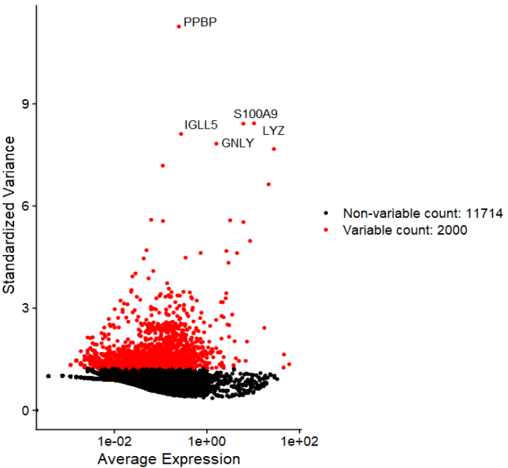
1、高变基因
- 可设置参数,加标签
|
|
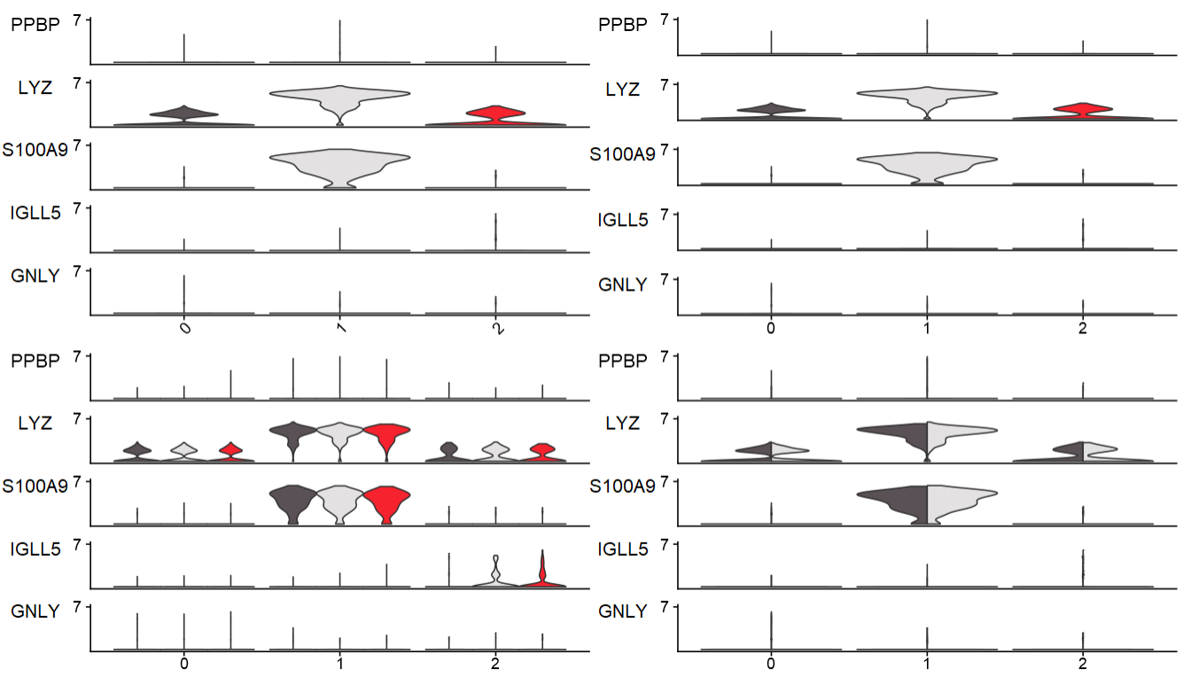
2、小提琴图
|
|
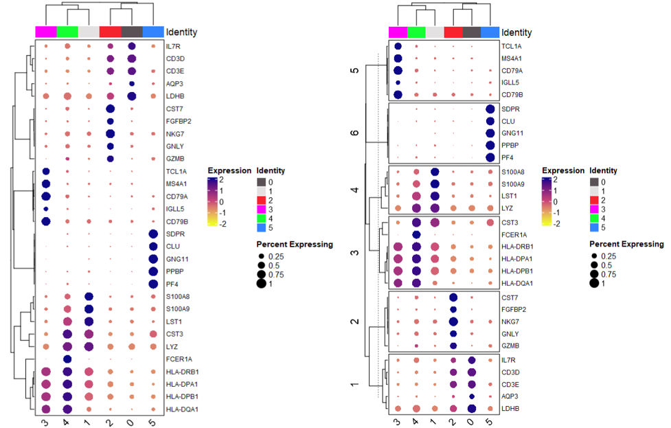
3、聚类点图
|
|
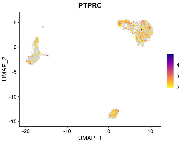
4、降维相关可视化
- (1)FeaturePlot_scCustom:低于特定阈值的基因不映射连续颜色
|
|
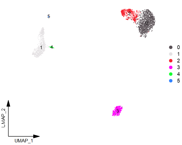
- (2)DimPlot_scCustom:迷你版坐标轴
|
|
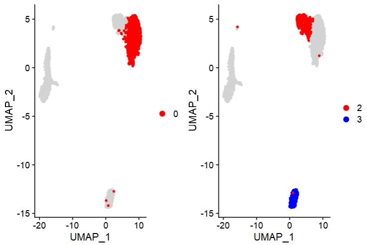
- (3)Cluster_Highlight_Plot:单独显示特定细胞群
|
|
5、自定义颜色
- (1)连续型变量:默认为
viridis_plasma_dark_high,其它可选包括viridis_plasma_light_highviridis_magma_dark_highviridis_magma_light_highviridis_inferno_dark_highviridis_inferno_light_highviridis_dark_highviridis_light_high
|
|

- (2)离散型变量:单变量-“dodgerblue”;双变量-NavyAndOrange();<36-“polychrome”;>36–“varibow”(shuffle)。其它包括
- alphabet (24)
- alphabet2 (24)
- glasbey (32)
- polychrome (36)
- stepped (24)
- ditto_seq (40)
- varibow (Dynamic)
|
|

|
|
