R包MARVEL是由牛津大学MRC Weatherall分子医学研究所团队开发的,用于分析单细胞水平的可变剪切事件。相关文章于2023年1月在Nucleic Acids Research期刊发表,在其github页面分享了MARVEL工具的分析流程,在此学习、记录如下。
- Pape:https://doi.org/10.1093/nar/gkac1260
- Github:https://github.com/wenweixiong/MARVEL
- Plate pipeline:https://wenweixiong.github.io/MARVEL_Plate.html
- Droplet pipeline:https://wenweixiong.github.io/MARVEL_Droplet.html
可变剪切
-
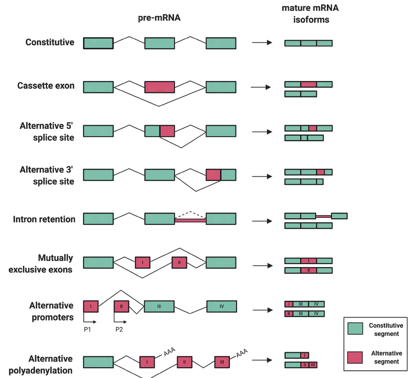
关于可变剪切(Alternative splicing,AS)的基础,可以参看一篇中文教程;其中关于基因结构组成,可以参考之前的笔记。
-
过去,针对Bulk RNA-seq数据的可变剪切分析工具已经有很多,例如之前学习的IsoformSwitchAnalyzeR包。MARVEL是个人目前了解到的第一个针对单细胞转录数据AS分析工具。
单细胞数据类型
- AS分析的核心是通过检测比对到splice junction位点的read(例如,跨越两个外显子)进行分析。
- 目前主流的单细胞测序技术主要分为Droplet-based 10X方法与Plate-based Smart-seq方法。
- 10X技术由于仅对cDNA的3’端部分进行测序,只能对该区域涉及的splice junction进行分析,且无法具体分析事件类型
- Smart-seq技术虽然通量低,但是全长转录本的单细胞测序原理,可以进行更为深入的AS分析。
一、Plate-based pipeline
1、上游分析
1.1 工作环境
两个同级的目录(1)basic:参考数据以及代码脚本 (2)proj1:具体的分析项目文件
- 后续分析均在
proj1/路径下操作
|
|
1.2 conda环境
|
|
1.2 准备数据
(1)测序数据
- 官方手册分析了如下数据集的 192个单细胞数据,以其中一个演示流程
|
|
(2)基因组数据
- 在 ./basic/gtf 目录下
- https://ftp.ebi.ac.uk/pub/databases/gencode/Gencode_human/release_31/
|
|
(3)教程数据
- 官方教程提供了各个分析步骤的示范文件,可供之后分析作为参考。
- http://datashare.molbiol.ox.ac.uk/public/wwen/MARVEL/Tutorial/Plate/Data.zip
|
|
1.3 分析步骤
1.3.1 单样本4步分析
(1)单样本STAR比对
将每个样本的Fastq文件使用STAR软件进行比对,产生每个splice junction count matrix
1 2# Reference less -SN ./Data/SJ/SJ.txt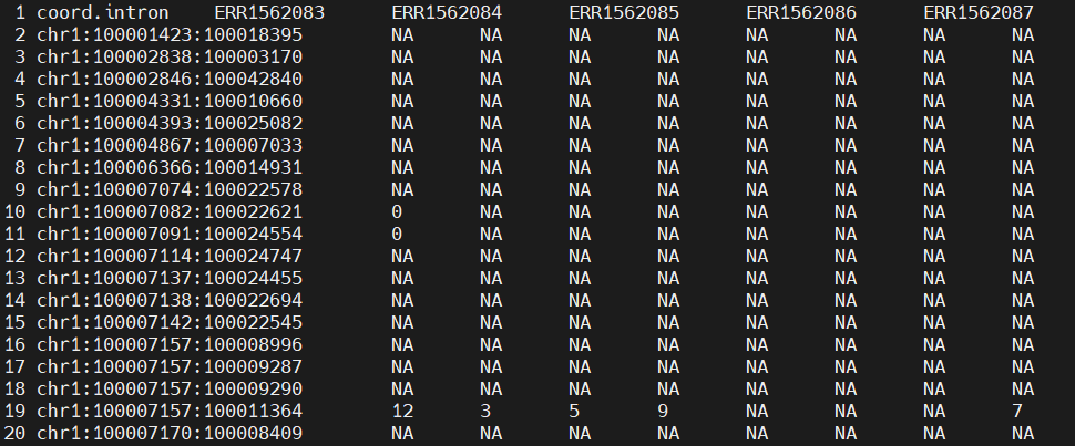
|
|
(2)单样本rMATs注释
根据上述比对BAM结果,注释出每个基因(转录本)涉及的可变剪切事件类型。使用rMATs软件,可注释出5种类型:SE、RI、MXE、A5SS、A3SS。
1 2 3 4 5 6 7find ./Data/rMATS/ -name *featureData.txt # ./Data/rMATS/SE/SE_featureData.txt # ./Data/rMATS/A3SS/A3SS_featureData.txt # ./Data/rMATS/MXE/MXE_featureData.txt # ./Data/rMATS/RI/RI_featureData.txt # ./Data/rMATS/A5SS/A5SS_featureData.txt less -SN ./Data/rMATS/SE/SE_featureData.txt
|
|
(3)单样本Intron矩阵
统计Reads对于每个内含子的比对情况,逐碱基累加作为比对结果。
1 2# reference less -SN Data/MARVEL/PSI/RI/Counts_by_Region.txt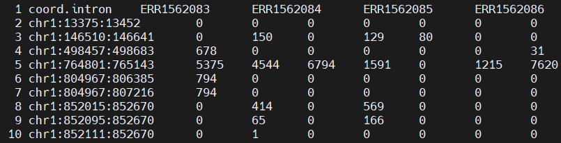
|
|
(4)单样本gene矩阵
最后需要对基因表达水平进行定量。教程推荐使用RSEM软件,并进行TPM类似的标准化处理
1
2
# reference less -SN ./Data/RSEM/TPM.txt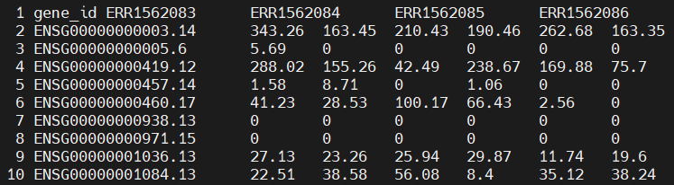
|
|
(1)如上,由于4步的分析过程中产生的中间数据可能超过数百兆;且SMART-seq往往涉及成百上千的细胞。为节约空间,可在每个样本分析完成后,删除不必要的数据。
1 2 3 4 5rm ./work/fq/${id}/${id}* rm ./work/star/${id}/*bam rm -rf ./work/rmats/${id}/tmp/* rm ./work/rsem/${id}/${id}.transcript.bam rm ./work/rsem/${id}/${id}.isoforms.results(2)多样本批量后台运行方式
1 2 3 4 5 6 7 8 9cat ../basic/single_sample_upstream.sh chmod u+x ../basic/single_sample_upstream.sh # 单样本测试 # ../basic/single_sample_upstream.sh ERR1562273 # parallel多线程批量运行 nohup parallel -j 5 ../basic/single_sample_upstream.sh {} ::: \ $(grep -v "sample" ./SJ_phenoData.txt | awk '{print $1}') \ 1> ./work/single_sample_upstream.log 2>&1 &
1.3.2 整合多样本结果
即分步整合上游4个步骤中的每个步骤的所有样本结果;均使用R语言完成
|
|
- step1: 汇总剪切位点矩阵
|
|
- step2:整理AS注释结果
- 这一步最为复杂,需要理解每一种剪切事件的定义以及正负链的差异
- 参考官方示意:https://wenweixiong.github.io/Splicing_Nomenclature
|
|
- step3:汇总intron矩阵
|
|
- 汇总gene矩阵
|
|
2、下游分析
后续根据教程提供的数据学习,需要安装的主要的MARVEL包以及其它辅助分析包,具体可参考教程。
|
|
2.1 创建marvel对象
需要准备七类文件,读入为R语言对象
- 样本表型data.frame:第一列名为sample.id
- 剪切位点计数矩阵:第一列名为coord.intron
- 剪切事件类型注释列表:由数据框包装而出的list,每个数据库至少包含tran_id与gene_id
- 内含子计数矩阵:第一列名为coord.intron
- 基因表达矩阵:经标准化处理(RPKM/FPKM/TPM),暂时不要log转换
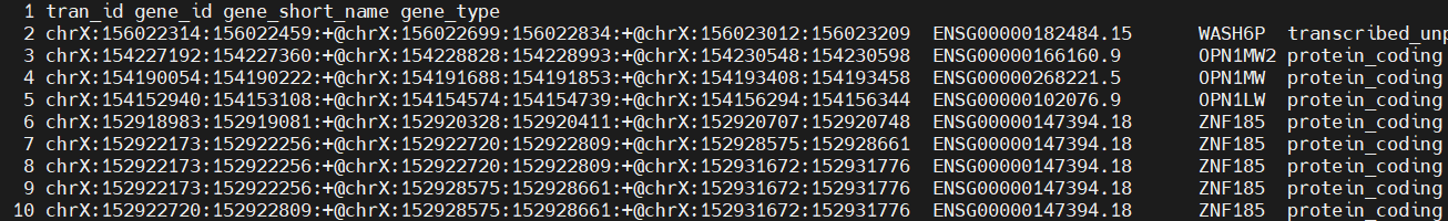
- 基因类型data.frame:至少包含3列,gene_id, gene_short_name, gene_type
- 上游分析所用到的GTF数据
|
|
2.2 预处理步骤
(1)基因表达log转换
|
|
(2)检测额外AS事件
|
|
(3)计算PSI值
计算一个基因对于特定剪切事件的PSI值,这是后续分析的基础
|
|
(4)保存中间结果
- 首先检查不同矩阵与对应的meta行列名信息一致
|
|
- 可进一步选取感兴趣的细胞群
|
|
- 保存中间结果,方便后续分析
|
|
2.3 细胞群AS特征分析
以其中84个iPSC细胞群进行演示
|
|
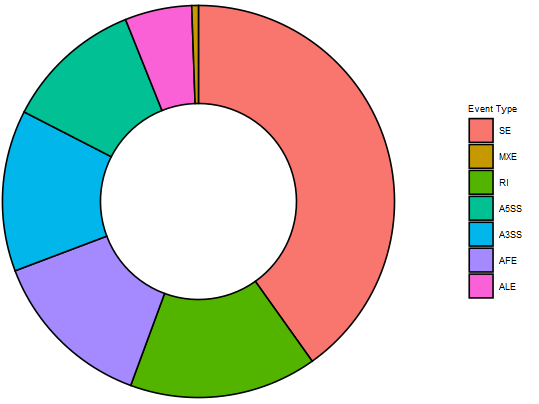
(1)AS类型占比
|
|
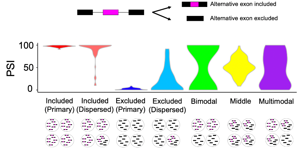
(2)AS modality
判断细胞群中每个基因的每种可变剪切的PSI分布类型,如下可分为7类
|
|
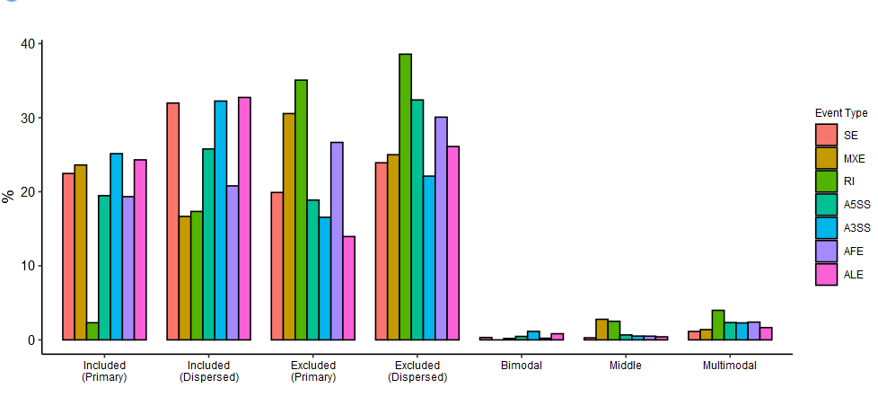
- 后续有两种统计方式:仅按modality分,同时按modality与AS type分。以后者作为演示
|
|
2.4 细胞群差异分析
(1)差异基因分析
|
|
(2)差异AS分析
|
|
(3)差异基因&AS分析
- 对差异可变剪切的基因执行基因表达差异分析
|
|
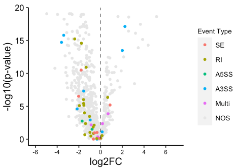
对于上述差异分析结果均可快速火山图,标记marker基因等
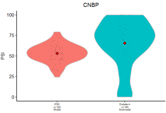
2.5 差异AS进阶分析
(1)差异PSI分类
- Explicit:明显的变化;Implicit:有限的变化;Restricted:微小的变化
|
|
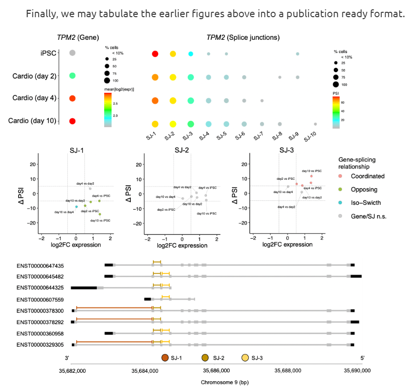
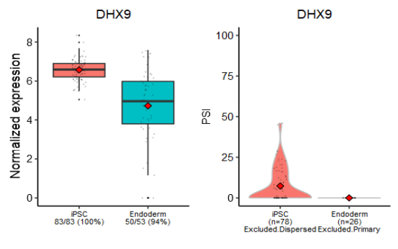
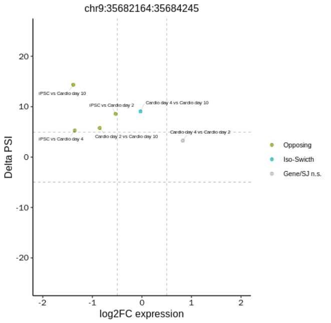
(2)差异基因与AS
- Coordinated:基因高表达,相应的PSI也增高;
- Opposing:基因表达与PSI变化方向相反;
- Isoform-switching :基因表达不变,PSI发生变化
- Complex:其它复杂情况
|
|
(3)NMD预测
- nonsense-mediated decay (NMD)无义介导的mRNA降解预测
- 相比对照组,观测组所剪切的外显子可能由于包含premature stop codons (PTCs),导致编码提前结束,从而进一步使得表达量降低。
- 本质上是对可产生PTC的可变剪切与下调基因取交集。
|
|
二、Drop-baed pipeline
1、上游分析
1.1 conda环境
|
|
1.2 下载数据
(1)测序数据
- 官方教程分析了GSE130731的4个10X单细胞测序结果,以其中的两个作为学习的示例(SRR9008752,SRR9008753)
- https://www.ncbi.nlm.nih.gov/geo/query/acc.cgi?acc=GSE130731
|
|
(2)基因组数据
还是在 ./basic/gtf 文件夹下,构建starsolo版本的索引文件。
cellranger软件及相关数据下载参考之前的笔记。
|
|
(3)教程数据
|
|
1.3 比对分析
(1)cellranger
使用cellranger软件初次比对产生bam文件,该软件用法可参考之前的笔记
|
|
(2)STARsolo
使用STAR软件针对单细胞数据的模式,分析其基因表达以及剪切位点矩阵
|
|
2、下游分析
2.1 整理比对结果
|
|
(1)Raw gene count
|
|
(2)Norm gene count
|
|
(3)Raw SJ count
|
|
(4)Cell dimension reduction
|
|
2.2 创建marvel对象
|
|
2.3 预处理步骤
- 筛选有效的剪切位点
|
|
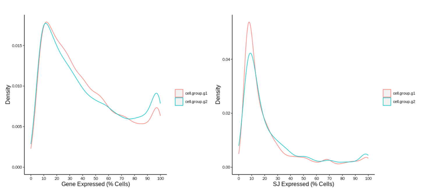
- 分析基因在细胞群的表达率以及SJ在细胞群的发生率
|
|
- 保存中间结果
|
|
2.4 SJ差异分析
(1)差异SJ与基因
|
|
(2)SJ与基因关系
|
|
- 降维可视化
|
|
2.5 特定基因分析
(1)分组表达
|
|
(2)组间差异
|
|
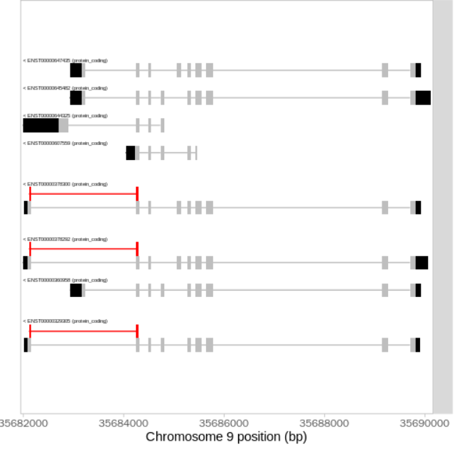
- 使用wiggleplotr包可视化某剪切位点在基因不同转录本的可视化
|
|