MAST,全称Model-based Analysis of Single-cell Transcriptomics,是2015年于Genome Biology发表的R包工具,主要用于单细胞数据的差异表达分析。参看官方教程,简单记录用法如下。
原始论文:https://genomebiology.biomedcentral.com/articles/10.1186/s13059-015-0844-5
Github:https://github.com/RGLab/MAST
官方手册:http://bioconductor.org/packages/release/bioc/vignettes/MAST/inst/doc/MAITAnalysis.html
1
|
BiocManager::install("MAST")
|
1
2
|
library(MAST)
library(tidyverse)
|
1、示例数据#
- 经细胞因子刺激前后的MAITs细胞的单细胞表达数据,使用MAST包分析其差异表达基因。
 1
 2
 3
 4
 5
 6
 7
 8
 9
10
11
12
13
14
15
16
17
18
19
20
21
22
23
24
25
26
27
28
|
data(maits, package='MAST')
dim(maits$expressionmat) #共96个细胞
# [1]    96 16302
maits$expressionmat[1:4,1:4]
head(maits$cdat) #细胞注释数据
head(maits$fdat) #基因注释数据

##整理表达矩阵,使用symbol作为基因名
idx = -which(duplicated(maits$fdat$symbolid))
maits$fdat = maits$fdat[idx,]
maits$fdat = maits$fdat[,-1]
rownames(maits$fdat) = maits$fdat$symbolid
maits$expressionmat = maits$expressionmat[,idx]
colnames(maits$expressionmat) = rownames(maits$fdat)

dim(maits$expressionmat)
# [1]    96 15077
maits$expressionmat[1:4,1:4]
#                     WASH7P    FAM138F LOC100132062 LOC100133331
# 1-MAIT-Stim-C05_S91      0 0.08406426    3.7158934     6.829215
# 1-MAIT-Stim-C07_S70      0 0.12432814    0.0000000     0.000000
# 1-MAIT-Stim-C08_S68      0 1.79077204    0.0000000     0.000000
# 1-MAIT-Stim-C10_S95      0 1.71369581    0.2141248     0.000000
head(maits$fdat)
#                 entrez     symbolid
# WASH7P          653635       WASH7P
# FAM138F         641702      FAM138F
# LOC100132062 100132062 LOC100132062
|
2、构建SingleCellAssay对象#
 1
 2
 3
 4
 5
 6
 7
 8
 9
10
11
12
13
14
15
16
17
18
19
20
21
22
23
24
25
26
|
sca = FromMatrix(t(maits$expressionmat), maits$cdat, maits$fdat)
## 方便演示,随机筛选出2000个基因
sca = sca[unique(sample(rownames(sca),2000)),]
dim(sca)
# [1] 16302    96

## (1) 目标分组
table(colData(sca)$condition)
# Stim Unstim
# 47     49
## 将Unstim设置为参考组
cond<-factor(colData(sca)$condition)
cond<-relevel(cond,"Unstim")
colData(sca)$condition<-cond

## (2) 考虑一个协变量因素
summary(colData(sca)$cngeneson)
#     Min.  1st Qu.   Median     Mean  3rd Qu.     Max.
# -0.17159 -0.02578  0.01408  0.00000  0.05943  0.15415

## (3) 模拟一个分类变量分组因素
set.seed(123)
colData(sca)$region = sample(letters[1:3], ncol(sca), replace=T)
table(colData(sca)$region)
# a  b  c
#32 31 33
|
3、回归分析#
- MAST做差异分析的主要优势在于可以校正多种协变量因素,如下演示几种常用的用法。
 1
 2
 3
 4
 5
 6
 7
 8
 9
10
11
12
13
14
15
16
17
18
19
20
21
22
23
|
## (1) 校正cngeneson协变量:默认参数
zlmCond <- zlm(~condition + cngeneson, sca,
    method="bayesglm", ebayes=TRUE)
summaryCond <- summary(zlmCond, doLRT='conditionStim')
summaryDt <- summaryCond$datatable
levels(summaryDt$contrast)
# [1] "conditionStim" "(Intercept)"   "cngeneson"

## (2) 校正cngeneson与region协变量:默认参数
zlmCond <- zlm(~condition + cngeneson + region, sca,
    method = "bayesglm", ebayes=TRUE)
summaryCond <- summary(zlmCond, doLRT='conditionStim')
summaryDt <- summaryCond$datatable
levels(summaryDt$contrast)
# [1] "conditionStim" "(Intercept)"   "cngeneson"     "regionb"       "regionc"

## (3) 校正cngeneson协变量,将region认为是随机因素
zlmCond <- zlm(~condition + cngeneson + (1|region), sca,
    method = "glmer", ebayes=FALSE)
summaryCond <- summary(zlmCond, doLRT='conditionStim')
summaryDt <- summaryCond$datatable
levels(summaryDt$contrast)
# [1] "conditionStim" "(Intercept)"   "cngeneson"
|
 1
 2
 3
 4
 5
 6
 7
 8
 9
10
11
12
13
14
15
16
17
18
19
20
21
22
23
|
df_pval = summaryDt %>%
    dplyr::filter(contrast=='conditionStim') %>%
    dplyr::filter(component=='H') %>%
    dplyr::select(primerid, `Pr(>Chisq)`)

df_logfc = summaryDt %>%
    dplyr::filter(contrast=='conditionStim') %>%
    dplyr::filter(component=='logFC') %>%
    dplyr::select(primerid, coef, ci.hi, ci.lo)

df_stat = dplyr::inner_join(df_logfc, df_pval) %>%
    dplyr::rename("symbol"="primerid") %>%
    dplyr::rename("pval"="Pr(>Chisq)","logFC"="coef") %>%
    dplyr::mutate("fdr" = p.adjust(pval)) %>%
    dplyr::arrange(fdr)
head(df_stat)
#    symbol     logFC      ci.hi      ci.lo         pval          fdr
# 1: NDUFV2  7.522343  8.8016689  6.2430166 2.586874e-18 5.109075e-15
# 2:   KIF9 -0.225052  0.1273536 -0.5774576 1.760028e-16 3.474294e-13
# 3:  DUSP1 -6.513010 -5.2606967 -7.7653235 8.668938e-15 1.710382e-11
# 4:    VCP  5.155219  6.2345839  4.0758540 1.530723e-13 3.018586e-10
# 5:   SARS  5.577095  6.8474645  4.3067258 1.216538e-12 2.397796e-09
# 6:  HSPD1  6.261077  7.6919267  4.8302277 1.969255e-12 3.879433e-09
|
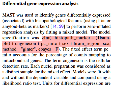
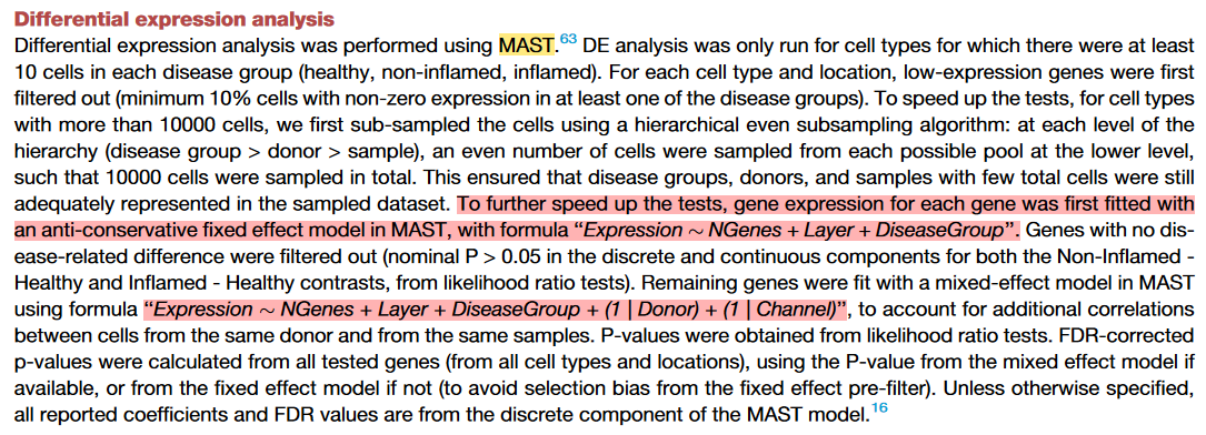
上述第3种差异分析方式在一些文献中经常提及,主要用于避免不同样本来源对差异分析造成的影响,例如下面两篇文章。
(1)The landscape of immune dysregulation in Crohn’s disease revealed through single-cell transcriptomic profiling in the ileum and colon
(2)Diverse human astrocyte and microglial transcriptional responses to Alzheimer’s pathology