- 原始论文:https://www.nature.com/articles/s41592-019-0667-5
- 官方手册:https://github.com/saeyslab/nichenetr
1
2
|
# install.packages("devtools")
devtools::install_github("saeyslab/nichenetr")
|
0、原理简介#
(1)NicheNet是2020年于Nature method提出的单细胞数据细胞通讯分析工具。相比于cellphoneDB等工具,NicheNet进一步考虑了受体被激活后的信号传导与下游靶基因的差异表达情况。
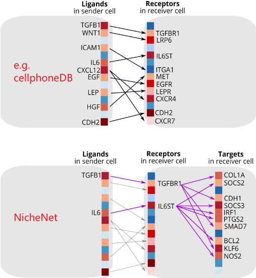
(2)如下图所示,NicheNet的核心思路是根据receiver cell的特定基因集,寻找最有可能的上游配体以及相应的sender cell。其中有如下要点
- 特定基因集,原文称为gene set of interest,即细胞通讯最终所影响的基因(target gene);一般表示receiver cell受外界影响因素而产生的差异表达基因(e.g. 造模前后、给药前后)。
- 根据上述特定基因集的定义,一般需要前后对照的单细胞数据才能进行NicheNet分析
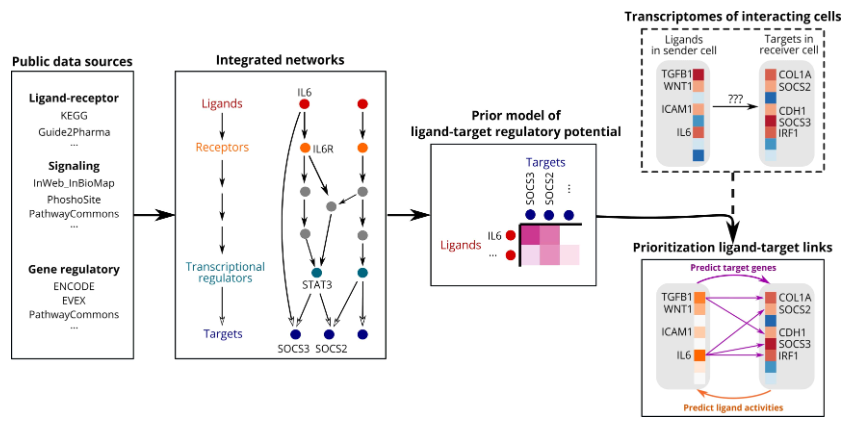
- NicheNet预测潜在上游配体的核心思路是计算配体所影响的下游基因与受体细胞所观测的特定基因集的相似性。如果相似性高,则认为是潜在的配体。
- 在分析时,仅根据所在细胞类型对于配/受体表达比例界定是否表达,之后的分析将不会再考虑其表达情况;
1、数据准备#
NicheNet基础分析时需要准备如下的3个输入数据。其由人类基因相关数据库整理而成;对于小鼠单细胞数据分析,可(1)直接将人基因名进行同源转换;(2)根据小鼠相关数据库,自己整理出下面的文件。
 1
 2
 3
 4
 5
 6
 7
 8
 9
10
|
ligand_target_matrix = readRDS("ligand_target_matrix.rds")
# target genes in rows, ligands in columns
dim(ligand_target_matrix)
# [1] 25345   688
ligand_target_matrix[1:4,1:4]
#                 CXCL1        CXCL2        CXCL3        CXCL5
# A1BG     0.0003534343 0.0004041324 0.0003729920 0.0003080640
# A1BG-AS1 0.0001650894 0.0001509213 0.0001583594 0.0001317253
# A1CF     0.0005787175 0.0004596295 0.0003895907 0.0003293275
# A2M      0.0006027058 0.0005996617 0.0005164365 0.0004517236
|
1
2
3
4
5
6
7
8
9
|
lr_network = readRDS("lr_network.rds")
dim(lr_network)
# [1] 12651     4
head(lr_network)
#    from    to         source database
# 1 CXCL1 CXCR2 kegg_cytokines     kegg
# 2 CXCL2 CXCR2 kegg_cytokines     kegg
# 3 CXCL3 CXCR2 kegg_cytokines     kegg
# 4 CXCL5 CXCR2 kegg_cytokines     kegg
|
 1
 2
 3
 4
 5
 6
 7
 8
 9
10
11
12
13
14
|
weighted_networks = readRDS("weighted_networks.rds")
# (1)interactions and their weights in the ligand-receptor + signaling network
head(weighted_networks$lr_sig)
#   from     to     weight
# 1 A1BG  ABCC6 0.42164389
# 2 A1BG   ACE2 0.10074109
# 3 A1BG ADAM10 0.09698978

# (2)interactions and their weights in the gene regulatory network
head(weighted_networks$gr)
#    from     to     weight
# 1  A1BG    A2M 0.02944793
# 2  AAAS   GFAP 0.02904173
# 3 AADAC CYP3A4 0.04215706
|
2、基础分析#
参考官方手册,可直接从单细胞表达矩阵开始分析;也可以基于Seurat格式进行分析。如下将采取后者进行学习。
1
2
3
|
library(nichenetr)
library(Seurat) # please update to Seurat V4
library(tidyverse)
|
(1)示例数据#
经LCMV感染前后的腹股沟淋巴结的单细胞测序数据,数据已完成细胞类型注释等分析。
https://zenodo.org/record/3531889/files/seuratObj.rds
分析目的:发现在LCMV感染后,哪些细胞类型的哪些配体参与到CD8 T细胞内的基因表达变化。
1
2
3
4
5
6
7
|
seuratObj = readRDS("seuratObj.rds")
table(seuratObj$celltype)
#   B CD4 T CD8 T    DC  Mono    NK  Treg
# 382  2562  1645    18    90   131   199
table(seuratObj$aggregate)
# LCMV   SS
# 3886 1141
|
(2)函数参数#
NicheNet的基础分析可由包装好的nichenet_seuratobj_aggregate()函数一次性完成,因此参数较多;下面简单介绍下其中重要的参数。
 1
 2
 3
 4
 5
 6
 7
 8
 9
10
11
12
13
14
15
16
17
18
19
20
21
|
nichenet_seuratobj_aggregate(
  seurat_obj = seuratObj, # Seurat对象,其active.ident需设置为细胞类型
  expression_pct = 0.10,  # 界定细胞类型是否表达配/受体的比例阈值,默认为0.1
  organism = "mouse", # 交代物种信息,默认为人类 c("human","mouse")
  #Group
  condition_colname = "aggregate",   # 交代分组的meta名
  condition_oi = "LCMV", condition_reference = "SS", # 交代实验组与对照组名
  # receiver
  receiver = "CD8 T",  # 交代receiver细胞类型
  geneset = "DE", # 判断特定基因集的方法,默认使用全部差异基因(oi/ref)c("DE","up","down")
  lfc_cutoff = 0.25, # 判断差异基因的阈值
  # sender
  sender = c("CD4 T","Treg", "Mono", "NK", "B", "DC"), #设置可能的sender cell
  top_n_targets = 200,  #每个ligand最多考虑200个target gene
  top_n_ligands = 20,   #给出最有可能的20个上游ligand
  cutoff_visualization = 0.33,  #设置可视化ligand-target scores的阈值
  # refer data
  ligand_target_matrix = ligand_target_matrix,
  lr_network = lr_network,
  weighted_networks = weighted_networks,
  )
|
receiver参数可以是多种细胞类型,会对每一种单独分析,将结果整合为list
sender参数设置为all时考虑所有细胞类型为sender,包括receiver(自分泌);设置为undefined时,则不考虑细胞类型。
(3)结果解读#
 1
 2
 3
 4
 5
 6
 7
 8
 9
10
11
12
13
14
15
16
17
18
19
20
21
22
23
24
25
26
27
|
Idents(seuratObj)="celltype"

ligand_target_matrix = readRDS("ligand_target_matrix.rds")
lr_network = readRDS("lr_network.rds")
weighted_networks = readRDS("weighted_networks.rds")

nichenet_output = nichenet_seuratobj_aggregate(
  seurat_obj = seuratObj,
  expression_pct = 0.10,
  organism = "mouse", #
  #Group
  condition_colname = "aggregate",
  condition_oi = "LCMV", condition_reference = "SS",
  # receiver
  receiver = "CD8 T",
  geneset = "DE",
  lfc_cutoff = 0.25,
  # sender
  sender = c("CD4 T","Treg", "Mono", "NK", "B", "DC"),
  top_n_ligands = 20,
  top_n_targets = 200,
  cutoff_visualization = 0.33,
  # refer data
  ligand_target_matrix = ligand_target_matrix,
  lr_network = lr_network,
  weighted_networks = weighted_networks,
  )
|
 1
 2
 3
 4
 5
 6
 7
 8
 9
10
11
12
13
14
15
16
17
|
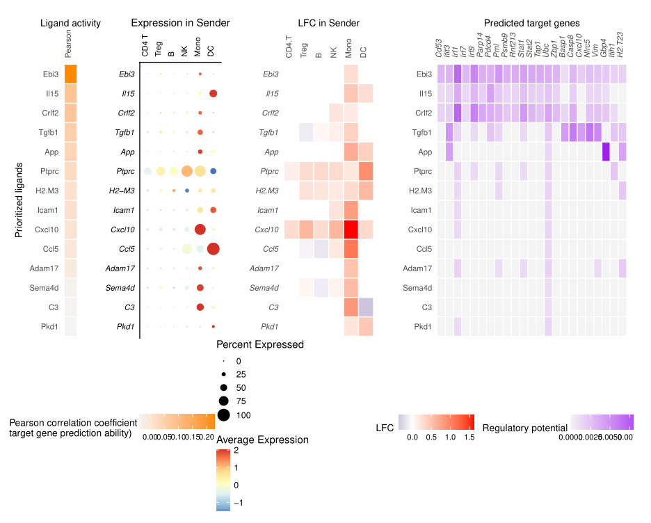
nichenet_output$ligand_activities
# # A tibble: 44 × 7
#    test_ligand auroc   aupr aupr_corrected  pearson  rank bona_fide_ligand
#    <chr>       <dbl>  <dbl>          <dbl>    <dbl> <dbl> <lgl>
#  1 Ebi3        0.690 0.211         0.128    0.229       1 FALSE
#  2 Il15        0.589 0.112         0.0286   0.0800      2 TRUE
#  3 Crlf2       0.555 0.122         0.0380   0.0757      3 FALSE
nichenet_output$top_ligands
#  [1] "Ebi3"   "Il15"   "Crlf2"  "Tgfb1"  "App"    "Ptprc"  "H2-M3"  "Icam1"
#  [9] "Cxcl10" "Ccl5"   "Cxcl11" "Adam17" "H2-T23" "Cxcl9"  "Cxcl16" "Sema4d"
# [17] "Calr"   "C3"     "Mif"    "Pkd1"

## 相关可视化
# ligand在不同细胞类型的表达
nichenet_output$ligand_expression_dotplot
# ligand在感染前后的差异表达
nichenet_output$ligand_differential_expression_heatmap
|
 1
 2
 3
 4
 5
 6
 7
 8
 9
10
11
12
13
14
15
16
17
18
19
20
21
|
# ligand-target score
nichenet_output$ligand_target_matrix %>% .[1:10,1:6]
nichenet_output$ligand_target_df %>% head
nichenet_output$top_targets

## 可视化
# ligand-target score热图
ichenet_output$ligand_target_heatma
# 靶基因在reciver细胞类型中的差异表达
DotPlot(seuratObj %>% subset(idents = "CD8 T"),
	features = nichenet_output$top_targets %>% rev(),
	split.by = "aggregate") +
	RotatedAxis()
VlnPlot(seuratObj %>% subset(idents = "CD8 T"),
	features = c("Zbp1","Ifit3","Irf7"),
	split.by = "aggregate",
	pt.size = 0,
	combine = FALSE)

## 上述的综合可视化
nichenet_output$ligand_activity_target_heatmap
|
 1
 2
 3
 4
 5
 6
 7
 8
 9
10
11
12
13
14
15
|
# ligand-receptor score
nichenet_output$ligand_receptor_matrix %>% .[1:10,1:6]
nichenet_output$ligand_receptor_df
nichenet_output$top_receptors

## 可视化
# ligand-receptor score热图
nichenet_output$ligand_receptor_heatmap
# receptor在receiver细胞类型的差异表达
nichenet_output$top_receptors

# ligand与receptor的注释来源可靠性
nichenet_output$ligand_receptor_matrix_bonafide
nichenet_output$ligand_receptor_df_bonafide
nichenet_output$ligand_receptor_heatmap_bonafide
|
1
2
|
nichenet_output$geneset_oi
nichenet_output$background_expressed_genes %>% length()
|
衍生可视化:可将ligand-target或者ligand-receptor的关系绘制成弦图,具体可参考:https://github.com/saeyslab/nichenetr/blob/master/vignettes/seurat_wrapper_circos.md
3、衍生分析#
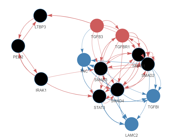
(1)信号路径可视化#
对基础分析结果得到的感兴趣上游配体与预测靶基因之间的信号传递过程进行网络可视化
- 数据准备:路径分析主要用到前两个文件;后3个文件主要用于数据来源/类型注释
 1
 2
 3
 4
 5
 6
 7
 8
 9
10
11
12
|
# https://zenodo.org/record/3260758/files/weighted_networks.rds
weighted_networks = readRDS("weighted_networks.rds")
# https://zenodo.org/record/3260758/files/ligand_tf_matrix.rds
ligand_tf_matrix = readRDS("ligand_tf_matrix.rds")


# https://zenodo.org/record/3260758/files/lr_network.rds
lr_network = readRDS("lr_network.rds")
# https://zenodo.org/record/3260758/files/signaling_network.rds
sig_network = readRDS("signaling_network.rds")
# https://zenodo.org/record/3260758/files/gr_network.rds
gr_network = readRDS("gr_network.rds")
|
 1
 2
 3
 4
 5
 6
 7
 8
 9
10
11
12
13
14
15
16
17
18
19
20
21
22
23
24
25
26
27
28
29
30
31
32
33
|
## 交代感兴趣的配体与受体
ligands_all = "TGFB3" # 可以是多个
targets_all = c("TGFBI","LAMC2","TNC")

## 分析/提取路径
active_signaling_network = get_ligand_signaling_path(
	ligand_tf_matrix = ligand_tf_matrix,
	ligands_all = ligands_all,
	targets_all = targets_all,
	weighted_networks = weighted_networks)
lapply(active_signaling_network, head)
# $sig
# # A tibble: 6 × 3
#   from  to    weight
#   <chr> <chr>  <dbl>
# 1 IRAK1 PELI2  1.54
# 2 IRAK1 SMAD3  0.608
# 3 IRAK1 STAT3  0.676

# $gr
# # A tibble: 6 × 3
#   from  to    weight
#   <chr> <chr>  <dbl>
# 1 SMAD1 TGFBI  0.0877
# 2 SMAD2 LAMC2  0.0587
# 3 SMAD2 TGFBI  0.0521

## 权重标准化
active_signaling_network_min_max = active_signaling_network
active_signaling_network_min_max$sig = active_signaling_network_min_max$sig %>%
	mutate(weight = ((weight-min(weight))/(max(weight)-min(weight))) + 0.75)
active_signaling_network_min_max$gr = active_signaling_network_min_max$gr %>%
	mutate(weight = ((weight-min(weight))/(max(weight)-min(weight))) + 0.75)
|
- 可视化(在linux环境好像不能绘制,window版本可以)
 1
 2
 3
 4
 5
 6
 7
 8
 9
10
11
12
13
|
## 转为dgr_graph对象
graph_min_max = diagrammer_format_signaling_graph(
	signaling_graph_list = active_signaling_network_min_max,
	ligands_all = ligands_all,
	targets_all = targets_all,
	sig_color = "indianred",
	gr_color = "steelblue")

## 可视化
DiagrammeR::render_graph(graph_min_max,
	output="visNetwork", # graph, visNetwork
	layout = "tree" # nicely, circle, tree, kk, and fr
	)
|
 1
 2
 3
 4
 5
 6
 7
 8
 9
10
11
12
13
14
15
16
17
18
19
20
21
22
23
24
25
26
27
28
29
30
31
32
33
34
35
36
37
38
39
40
41
42
43
44
45
46
47
48
49
50
51
|
## 边edge信息(权重)
bind_rows(active_signaling_network$sig %>% mutate(layer = "signaling"),
          active_signaling_network$gr %>% mutate(layer = "regulatory")) %>% head
# # A tibble: 6 × 4
#   from  to    weight layer
#   <chr> <chr>  <dbl> <chr>
# 1 IRAK1 PELI2 1.54   signaling
# 2 IRAK1 SMAD3 0.0608 signaling
# 3 IRAK1 STAT3 0.676  signaling

## 边edge注释来源信息
data_source_network = infer_supporting_datasources(
	signaling_graph_list = active_signaling_network,
	lr_network = lr_network,
	sig_network = sig_network,
	gr_network = gr_network)
head(data_source_network)
# # A tibble: 6 × 5
#   from  to    source            database       layer
#   <chr> <chr> <chr>             <chr>          <chr>
# 1 SMAD1 TGFBI regnetwork_source regnetwork     regulatory
# 2 SMAD1 TGFBI Remap_5           Remap          regulatory
# 3 SMAD2 LAMC2 harmonizome_CHEA  harmonizome_gr regulatory

## 节点node类型(4种)
all_genes = data_source_network[,c("from","to")] %>%
  as.matrix() %>% reshape2::melt() %>% .[,3] %>% unique()
specific_annotation_tbl = bind_rows(
  tibble(gene = ligands_all, annotation = "ligand"),
  tibble(gene = targets_all, annotation = "target"),
  tibble(gene = all_genes %>%
           setdiff(c(targets_all,ligands_all)) %>%
           intersect(lr_network$to %>% unique()),
         annotation = "receptor"),
  tibble(gene = all_genes %>%
           setdiff(c(targets_all,ligands_all)) %>%
           intersect(gr_network$from %>% unique()) %>%
           setdiff(all_genes %>% intersect(lr_network$to %>% unique())),
         annotation = "transcriptional regulator"))
non_specific_annotation_tbl = tibble(
  gene = all_genes %>% setdiff(specific_annotation_tbl$gene),
  annotation = "signaling mediator")
bind_rows(specific_annotation_tbl,non_specific_annotation_tbl) %>% count(annotation)
# # A tibble: 5 × 2
#   annotation                    n
#   <chr>                     <int>
# 1 ligand                        1
# 2 receptor                      1
# 3 signaling mediator            7
# 4 target                        3
# 5 transcriptional regulator     1
|
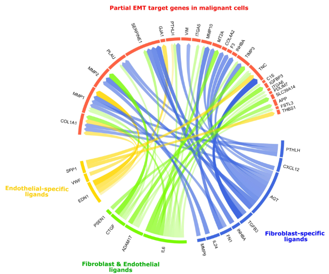
(2)自定义基因集#
分析场景:在头颈部鳞状细胞癌单细胞数据中,在成纤维细胞群中发现可诱导肿瘤细胞pEMT程序基因集表达的ligand。
 1
 2
 3
 4
 5
 6
 7
 8
 9
10
|
# ligand-target
ligand_target_matrix = readRDS("ligand_target_matrix.rds")
# ligand-receptor
lr_network = readRDS("lr_network.rds")

# 单细胞数据
hnscc_expression = readRDS("hnscc_expression.rds")
expression = hnscc_expression$expression
sample_info = hnscc_expression$sample_info # contains meta-information about the cells
tumors_remove = c("HN10","HN","HN12", "HN13", "HN24", "HN7", "HN8","HN23")
|
 1
 2
 3
 4
 5
 6
 7
 8
 9
10
11
12
13
14
15
16
17
|
## 成纤维细胞表达信息
CAF_ids = sample_info %>%
	filter(`Lymph node` == 0 & !(tumor %in% tumors_remove) & `non-cancer cell type` == "CAF") %>%
	pull(cell) #404
expressed_genes_CAFs = expression[CAF_ids,] %>%
	apply(2,function(x){10*(2**x - 1)}) %>%
	apply(2,function(x){log2(mean(x) + 1)}) %>%
	.[. >= 4] %>% names() # 6706

## 肿瘤恶性细胞表达信息
malignant_ids = sample_info %>%
	filter(`Lymph node` == 0 & !(tumor %in% tumors_remove) & `classified  as cancer cell` == 1) %>%
	pull(cell) #1388
expressed_genes_malignant = expression[malignant_ids,] %>%
	apply(2,function(x){10*(2**x - 1)}) %>%
	apply(2,function(x){log2(mean(x) + 1)}) %>%
	.[. >= 4] %>% names() # 6351
|
1
2
3
4
5
6
7
|
# pEMT基因集(靶基因)
pemt_geneset = readr::read_tsv("pemt_signature.txt", col_names = "gene") %>%
	pull(gene) %>% .[. %in% rownames(ligand_target_matrix)]

# 背景基因集(受体细胞表达)
background_expressed_genes = expressed_genes_malignant %>%
	.[. %in% rownames(ligand_target_matrix)]
|
 1
 2
 3
 4
 5
 6
 7
 8
 9
10
11
12
|
# 在CAF里表达的ligand
ligands = lr_network %>% pull(from) %>% unique()
expressed_ligands = intersect(ligands,expressed_genes_CAFs)
# 在tumor里表达的receptor
receptors = lr_network %>% pull(to) %>% unique()
expressed_receptors = intersect(receptors,expressed_genes_malignant)

# 符合最低条件的候选ligand-receptor pair
potential_ligands = lr_network %>%
	filter(from %in% expressed_ligands & to %in% expressed_receptors) %>%
	pull(from) %>% unique()
head(potential_ligands)
|
 1
 2
 3
 4
 5
 6
 7
 8
 9
10
11
|
ligand_activities = predict_ligand_activities(
	geneset = pemt_geneset,
	background_expressed_genes = background_expressed_genes,
	ligand_target_matrix = ligand_target_matrix,
	potential_ligands = potential_ligands)

ligand_activities %>% arrange(-pearson)
best_upstream_ligands = ligand_activities %>% top_n(20, pearson) %>%
	arrange(-pearson) %>% pull(test_ligand)
head(best_upstream_ligands)
# [1] "PTHLH"  "CXCL12" "AGT"    "TGFB3"  "IL6"    "INHBA"
|
- step6 根据Top20 ligand预测基因是否为pEMT相关基因
 1
 2
 3
 4
 5
 6
 7
 8
 9
10
11
12
13
14
15
16
17
18
19
20
21
22
23
24
25
|
k = 3 # 3-fold
n = 5 # 2 rounds
pemt_gene_predictions_top20_list = seq(n) %>%
	lapply(assess_rf_class_probabilities, folds = k,
		geneset = pemt_geneset, background_expressed_genes = background_expressed_genes,
		ligands_oi = best_upstream_ligands, ligand_target_matrix = ligand_target_matrix)

target_prediction_performances_cv = pemt_gene_predictions_top20_list %>%
	lapply(classification_evaluation_continuous_pred_wrapper) %>%
	bind_rows() %>% mutate(round=seq(1:nrow(.)))
dim(target_prediction_performances_cv)
# [1]  5 11

# 预测Top 5%的基因中 根据真实标签的两类基因的均分
target_prediction_performances_discrete_cv %>%
	filter(true_target) %>% .$fraction_positive_predicted %>% mean()
## [1] 0.25
target_prediction_performances_discrete_cv %>%
	filter(!true_target) %>% .$fraction_positive_predicted %>% mean()
## [1] 0.04769076
# fisher's test
target_prediction_performances_discrete_fisher = pemt_gene_predictions_top20_list %>%
	lapply(calculate_fraction_top_predicted_fisher, quantile_cutoff = 0.95)
target_prediction_performances_discrete_fisher %>% unlist() %>% mean()
## [1] 5.647773e-10
|
(3)单细胞配体活性#
假设:对于一个单细胞表达信息,如果sender配体的下游receiver靶基因高表达(相较其它细胞);则推测该配体有较高的活性。
分析数据同上面的肿瘤数据,并且分析过程中一直到确定候选ligand-receptor步骤一致(step1~4)
- step5:计算单细胞配体活性(receiver细胞中受sender cell配体调控的活性)
 1
 2
 3
 4
 5
 6
 7
 8
 9
10
11
12
13
14
15
16
17
18
19
20
21
22
23
24
25
26
27
28
|
# 对受体细胞表达信息进行标准化
expression_scaled = expression[malignant_ids,background_expressed_genes] %>% scale_quantile()

# 示例10个细胞进行分析
malignant_hn5_ids = sample_info %>% filter(tumor == "HN5") %>%
	filter(`Lymph node` == 0) %>% filter(`classified  as cancer cell` == 1)  %>%
	pull(cell) %>% head(10)

# 计算每个细胞对于所有候选配体的受调控活性
ligand_activities = predict_single_cell_ligand_activities(
	cell_ids = malignant_hn5_ids,
	expression_scaled = expression_scaled,
	ligand_target_matrix = ligand_target_matrix,
	potential_ligands = potential_ligands) # 131
dim(ligand_activities)
# [1] 1310    5
head(ligand_activities)
# # A tibble: 6 × 5
#   setting                 test_ligand auroc   aupr pearson
#   <chr>                   <chr>       <dbl>  <dbl>   <dbl>
# 1 HNSCC5_p3_HNSCC5_P3_E03 HGF         0.538 0.0310  0.0233
# 2 HNSCC5_p3_HNSCC5_P3_E03 TNFSF10     0.529 0.0292  0.0144
# 3 HNSCC5_p3_HNSCC5_P3_E03 TGFB2       0.551 0.0391  0.0343

## 对配体活性标准化
normalized_ligand_activities = normalize_single_cell_ligand_activities(ligand_activities)
dim(normalized_ligand_activities)
# [1]  10 132
|
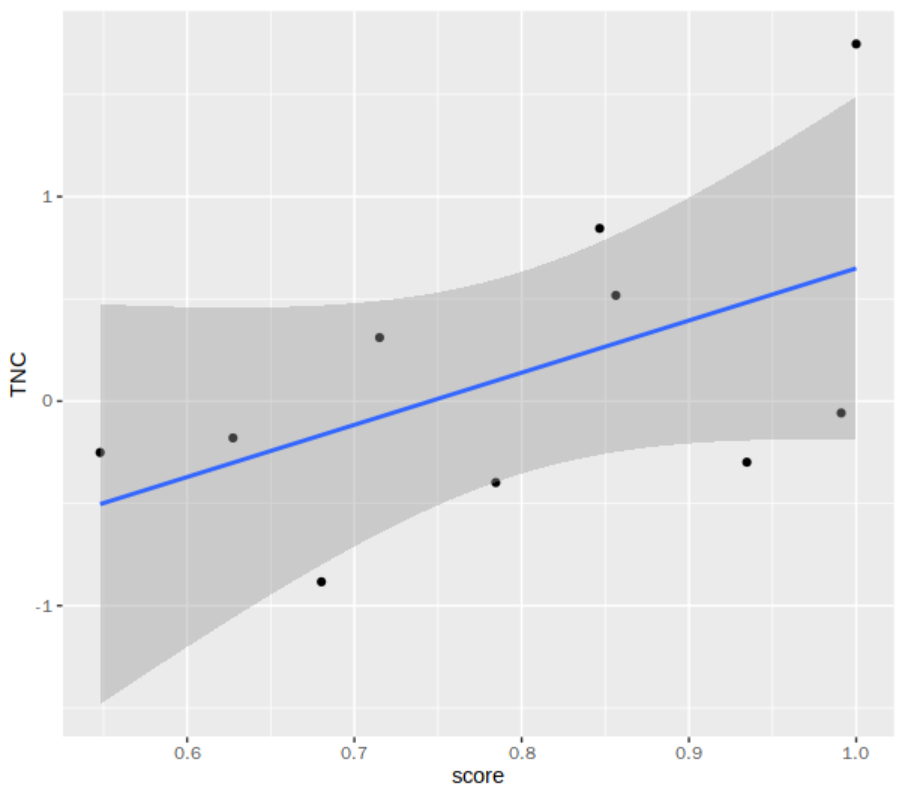
- step6:计算细胞配体活性与目标基因表达活性的相关性
1
2
3
4
5
6
7
8
|
cell_scores_tbl = tibble(
	cell = malignant_hn5_ids,
	score = expression_scaled[malignant_hn5_ids,"TGFBI"])
## 配体TNC活性与TGFB1配体表达的相关性
inner_join(cell_scores_tbl,normalized_ligand_activities) %>%
	ggplot(aes(score,TNC)) +
	geom_point() +
	geom_smooth(method = "lm")
|