cellphonedb是基于配受体对表达水平,分析单细胞数据中不同细胞类型间相互作用的Python工具。其于2020年在nature protocols发表,目前工具包版本以更新到3.1.0,配受体数据库已更新到4版本。如下将简单学习该软件的用法及结果可视化方法。

1、输入数据#
如下图所示,目前cellphonedb可主要实现三种分析模式。第一种直接分析细胞对之间配受体表达水平,第二种方式在前者基础上进一步计算显著P值。第三种则结合了细胞类型的差异基因。
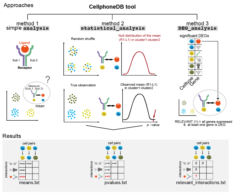
此次主要学习第二种分析模式,需要提供两类文件:单细胞表达矩阵,细胞类型注释结果。
- 单细胞表达矩阵
- (1)支持格式包括:
.h5ad(scannpy),10X三文件(mtx/barcode/features),以及txt等纯文本;对于大型单细胞数据,推荐使用前两者;
- (2)推荐使用标准化后的count标准矩阵,不需要scale归一化处理;
- (3)该工具仅支持人类基因名(ensembl, symbol),其它物种需要同源转换。
- 细胞类型注释结果
- (1)包含两列信息的文本文件,可支持
.csv, .txt,.tsv等
- (2)第一列的列名是Cell,对应表达矩阵的细胞名;第二列的列名是cell_type,表示注释细胞类型。
2、示例数据#
 1
 2
 3
 4
 5
 6
 7
 8
 9
10
11
12
13
14
15
16
17
18
19
20
21
22
23
24
25
26
27
28
29
30
31
32
33
34
35
|
library(Seurat)
library(tidyverse)

# https://support.10xgenomics.com/single-cell-gene-expression/datasets/1.1.0/pbmc3k
count = Read10X("filtered_gene_bc_matrices/hg19/")
sce = CreateSeuratObject(count)

sce = sce %>%
  NormalizeData() %>%
  FindVariableFeatures(nfeatures = 2000) %>%
  ScaleData()
sce = sce %>%
  RunPCA() %>%
  RunUMAP(dims = 1:30) %>%  #RunTSNE
  FindNeighbors(dims = 1:30) %>%
  FindClusters(resolution = 0.1)
table(sce$seurat_clusters)
#    0    1    2    3    4
# 1201  684  450  351   14

## (1) 重新保存10X三文件,prepared_10X文件夹中
dir.create("prepared_10x")
writeMM(sce@assays$RNA@data, file = 'prepared_10x/matrix.mtx')
write(x = rownames(sce@assays$RNA@data), file = "prepared_10x/features.tsv")
write(x = colnames(sce@assays$RNA@data), file = "prepared_10x/barcodes.tsv")

## (2) 保存细胞类型注释结果
sce$cell_type = paste0("cluster",sce$seurat_clusters)
sce$Cell = rownames(sce@meta.data)
df = sce@meta.data[, c('Cell', 'cell_type')]
write.table(df, file ='prepared_meta.tsv',
            sep = '\t', quote = F, row.names = F)

## (3) 保存当前seurat对象,用于扩展可视化
saveRDS(sce, file = "sce.rds")
|
将上述的结果(1个文件夹,2个文件)保存到后面的cellphonedb分析环境
3、cellphonedb分析#
 1
 2
 3
 4
 5
 6
 7
 8
 9
10
11
12
13
14
15
16
17
18
19
20
|
## python版本建议使用3.7
conda create -n cellphonedb python=3.7 -y
conda activate cellphonedb

conda install -c r r-base rpy2 -y
conda install r-pheatmap r-ggplot2 -y
conda install -c conda-forge markupsafe=2.0.1 -y
pip install cellphonedb

cellphonedb --help
# Commands:
#   database
#   method
#   plot
#   query
cellphonedb method --help
# Commands:
#   analysis
#   degs_analysis
#   statistical_analysis
|
如上,cellphonedb工具提供4个子命令,其中method用于细胞通讯分析的方法选择。
后续分析选择statistical_analysis模式,用于计算P值
1
2
3
4
5
6
|
cellphonedb method statistical_analysis  \
--output-path pbmc_out \
--counts-data hgnc_symbol  \
--threshold 0.1 \
--threads 10 \
prepared_meta.tsv  prepared_10x
|
该命令有较多参数可以设置,具体可参考官方手册。如上所示列出了觉得比较重要的4个参数。
--output-path :输出文件夹名,默认为out
--counts-data:表达矩阵基因基因名格式,默认为ensembl
--threshold:只有细胞类型的相应配受体表达百分比超过阈值才会分析,默认为0.1
--threads:多线程设置,默认为4
1
2
|
ls ./pbmc_out
# deconvoluted.txt  means.txt  pvalues.txt  significant_means.txt
|
如上结果里, means.txt与pvalues.txt表示两两细胞类型之间配受体对的平均表达水平与显著性P值。
significant_means.txt结合上述两个结果表示具有显著意义(至少在一种)的两两细胞类型之间配受体对的平均表达水平。
如下所示,考虑到配受体对的有向性,对于同一配受体对,会分析所有的细胞类型组合(n*n)可能。
id_cp_interaction、interacting_pair表示配受体对的代号与组成;
partner_a、gene_a表示组成A的蛋白标识符、基因名;同理表示组成B;
receptor_a 表示组成A是否为受体;其它列含义可参看官方手册。
 1
 2
 3
 4
 5
 6
 7
 8
 9
10
11
12
13
14
15
16
17
18
19
20
21
22
23
24
25
26
27
28
29
30
31
32
33
34
35
36
37
38
39
40
|
sig_m = read.table("./pbmc_out/significant_means.txt", sep="\t", header=T, check.names=F)
t(sig_m[1,])
#                     1
# id_cp_interaction   "CPI-SS0E292C126"
# interacting_pair    "KLRB1_CLEC2D"
# partner_a           "simple:Q12918"
# partner_b           "simple:Q9UHP7"
# gene_a              "KLRB1"
# gene_b              "CLEC2D"
# secreted            "False"
# receptor_a          "True"
# receptor_b          "True"
# annotation_strategy "curated"
# is_integrin         "False"
# rank                "0.04"
# cluster0|cluster0   NA
# cluster0|cluster1   NA
# cluster0|cluster2   NA
# cluster0|cluster3   NA
# cluster0|cluster4   NA
# cluster1|cluster0   NA
# cluster1|cluster1   NA
# cluster1|cluster2   NA
# cluster1|cluster3   NA
# cluster1|cluster4   NA
# cluster2|cluster0   "0.291"
# cluster2|cluster1   NA
# cluster2|cluster2   NA
# cluster2|cluster3   NA
# cluster2|cluster4   NA
# cluster3|cluster0   NA
# cluster3|cluster1   NA
# cluster3|cluster2   NA
# cluster3|cluster3   NA
# cluster3|cluster4   NA
# cluster4|cluster0   NA
# cluster4|cluster1   NA
# cluster4|cluster2   NA
# cluster4|cluster3   NA
# cluster4|cluster4   NA
|
4、结果可视化#
4.1 cellphonedb可视化#
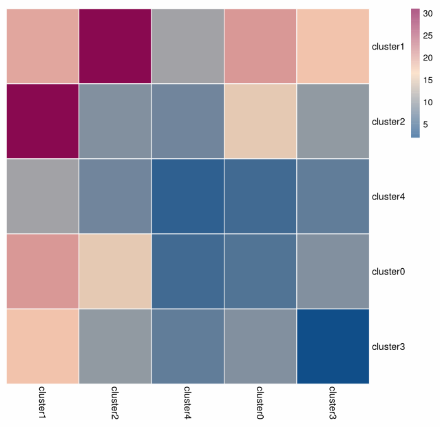
- 细胞类型间通讯热图,需要提供cellphonedb分析结果路径以及细胞类型注释结果
 1
 2
 3
 4
 5
 6
 7
 8
 9
10
|
cellphonedb plot heatmap_plot \
--pvalues-path ./pbmc_out/pvalues.txt \
--output-path ./pbmc_out \
--count-name heatmap_count.pdf \
--log-name heatmap_log_count.pdf \
--count-network-name count_network.txt \
--interaction-count-name interaction_count.txt \
./prepared_meta.tsv

# 根据是否log转换,会产生两张热图
|
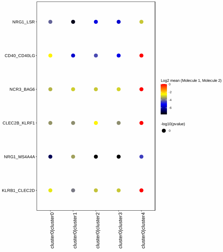
- 配受体对的点图,需要提供cellphonedb分析结果路径
 1
 2
 3
 4
 5
 6
 7
 8
 9
10
11
12
13
14
15
16
17
18
19
20
21
22
23
|
# 默认将所有配受体对的所有细胞类型组合进行可视化
cat rows.txt
# KLRB1_CLEC2D
# NRG1_MS4A4A
# CLEC2B_KLRF1
# NCR3_BAG6
# CD40_CD40LG
# NRG1_LSR

cat columns.txt
# cluster0|cluster0
# cluster0|cluster1
# cluster0|cluster2
# cluster0|cluster3
# cluster0|cluster4

cellphonedb plot dot_plot \
--means-path ./pbmc_out/means.txt \
--pvalues-path ./pbmc_out/pvalues.txt \
--output-path ./pbmc_out \
--output-name plot.pdf \
--rows rows.txt \
--columns columns.txt
|
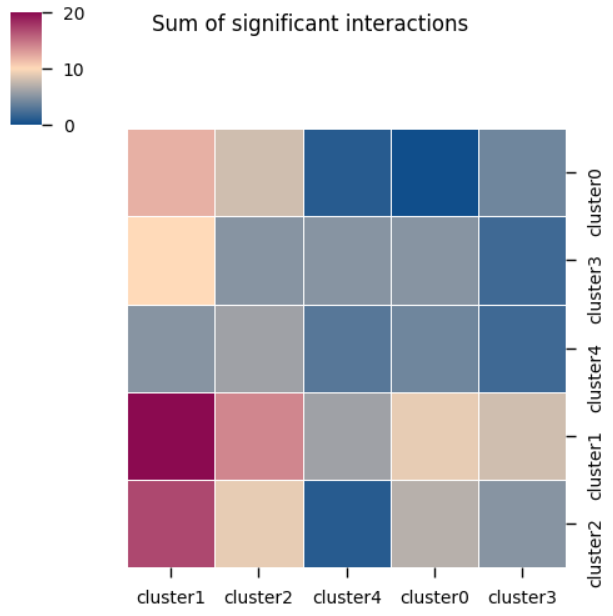
4.2 ktplotspy可视化#
上述cellphonedb提供的可视化方法较为简单,难以调整绘图细节。ktplotspy工具包可针对cellphonedb分析结果提供较为丰富的绘图方案。由于依赖包冲突,需要单独为ktplotspy单独创建一个conda环境。
1
2
3
4
|
conda create -n cellphonedb_plot python notebook -y
conda install -c bioconda r-seurat bioconductor-singlecellexperiment
conda install -c bioconda anndata anndata2ri
pip install ktplotspy
|
后续在jupyter notebook中操作、分析
- (2)导入数据:seurat对象转为anndata格式,并读入cellphonedb分析结果
1
2
3
4
5
6
7
8
|
import os
import anndata as ad
import pandas as pd
import ktplotspy as kpy
import matplotlib.pyplot as plt
import anndata2ri
anndata2ri.activate()
%load_ext rpy2.ipython
|
1
2
3
4
|
%%R
library(Seurat)
sce = readRDS("sce.rds")
sce
|
1
2
3
4
|
%%R -o anndata
#convert the Seurat object to a SingleCellExperiment object
anndata <- as.SingleCellExperiment(sce)
anndata
|
1
2
3
4
5
6
7
8
9
|
anndata
# AnnData object with n_obs × n_vars = 2700 × 32738
#     obs: 'orig.ident', 'nCount_RNA', 'nFeature_RNA', 'RNA_snn_res.0.1', 'seurat_clusters', 'cell_type', 'Cell', 'ident'
#     obsm: 'X_pca', 'X_umap'
#     layers: 'logcounts'

means = pd.read_csv('pbmc_out/means.txt', sep = '\t')
pvals = pd.read_csv('pbmc_out/pvalues.txt', sep = '\t')
decon = pd.read_csv('pbmc_out/deconvoluted.txt', sep = '\t')
|
1
2
3
4
5
6
7
8
|
kpy.plot_cpdb_heatmap(
        adata=adata,
        pvals=pvals,
        celltype_key="cell_type",
        figsize = (5,5),
        # symmetrical = False,
        title = "Sum of significant interactions"
    )
|
 1
 2
 3
 4
 5
 6
 7
 8
 9
10
11
12
13
14
15
16
|
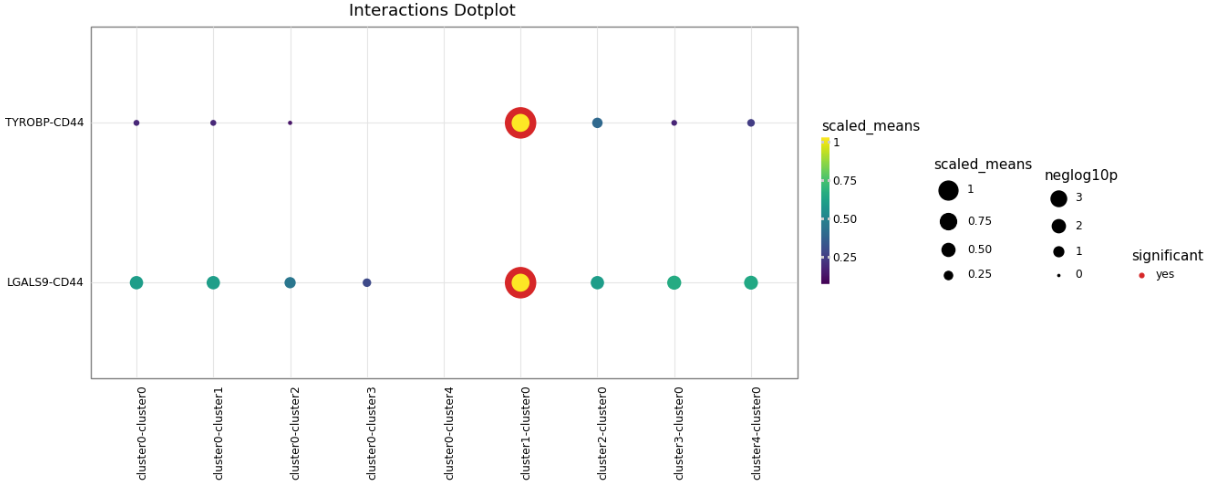
kpy.plot_cpdb(
        adata=adata,
        cell_type1="cluster0",
        # cell_type1="cluster[0,1]",   #  this means culster0 and cluster1
        cell_type2=".", # this means all cell-types
        means=means,
        pvals=pvals,
        celltype_key="cell_type",
        genes=["CD44"],
        figsize = (10,5),
        # highlight_col = "red",
        # highlight_size = 1,  将所有显著的配受体对标识圆环的宽度相同
        default_style = True,
        title = "Interactions Dotplot"
    )
# cell_type1与cell_type2并无先后顺序的区别
|
 1
 2
 3
 4
 5
 6
 7
 8
 9
10
11
12
|
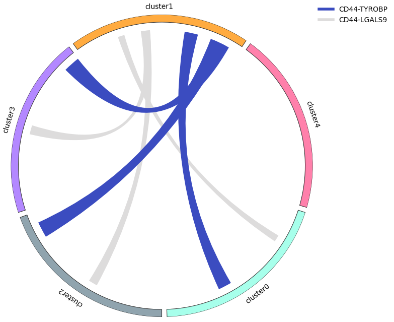
kpy.plot_cpdb_chord(
        adata=adata,
        cell_type1=".",
        cell_type2=".",
        means=means,
        pvals=pvals,
        deconvoluted=decon,
        celltype_key="cell_type",
        genes=["CD44"],
        edge_cmap=plt.cm.coolwarm,
        figsize=(6,6)
    )
|
1
2
3
4
5
6
7
8
9
|
## 可设置face_col_dict参数,修改每个条带的颜色
face_col_dict={
    "cluster0": "brown",
    "cluster1": "grey",
    "cluster2": "orange",
    "cluster3": "pink",
    "cluster4": "cyan",
},
edge_col_dict={"CD44-TYROBP": "red", "CD44-LGALS9": "blue"}
|