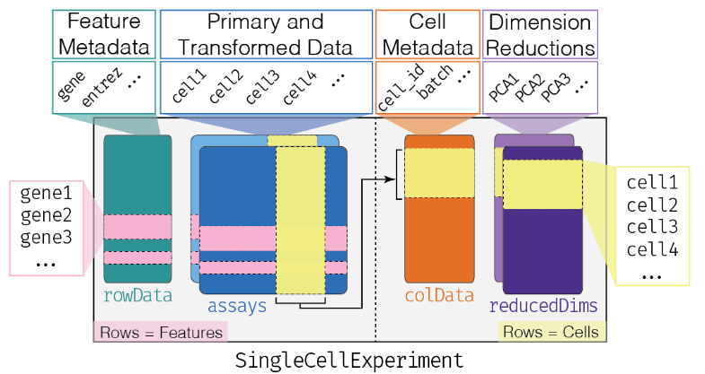
SingleCellExperiment是通过SingleCellExperiment包创建的单细胞数据分析对象,已有几十个单细胞R包支持。
其衍生自SummarizedExperiment,之前在GEO数据挖掘学习时,了解过相关知识,主要是assay与pData两个函数的使用。
- 参考文章:https://osca.bioconductor.org/data-infrastructure.html
0、创建sce#
 1
 2
 3
 4
 5
 6
 7
 8
 9
10
11
12
13
14
15
16
17
18
19
20
21
22
23
24
25
26
|
library(tidyverse)
library(SingleCellExperiment)
## 表达矩阵
# https://www.ncbi.nlm.nih.gov/geo/download/?acc=GSE81861&format=file&file=GSE81861%5FCRC%5FNM%5Fepithelial%5Fcells%5FCOUNT%2Ecsv%2Egz
nm_count <- read.csv("GSE81861_CRC_NM_epithelial_cells_COUNT.csv") %>%
tibble::column_to_rownames("X") %>%
as.matrix()
rownames(nm_count) <- sapply(strsplit(rownames(nm_count),"_"),"[",2)
colnames(nm_count) <- sapply(strsplit(colnames(nm_count),"_"),"[",1)
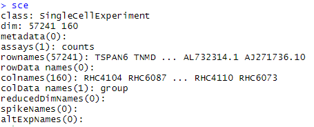
dim(nm_count)
# [1] 57241 160
nm_count[1:4,1:4]
# RHC4104 RHC6087 RHL2880 RHC5949
# TSPAN6 0 428 66 141
# TNMD 0 0 0 0
# DPM1 0 179 0 1
# SCYL3 465 0 0 0
## metadata
group.dat <- data.frame(group=rep("nomal",ncol(nm_count)))
## 创建sce
sce <- SingleCellExperiment(assays = list(counts = nm_count),
colData = group.dat)
sce
|
1、assay结构#
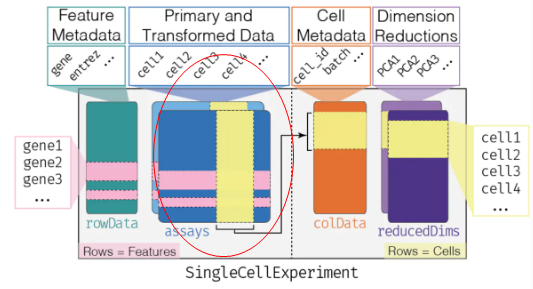
assays 中最基本的是列为sample,行为feature(一般是gene)的表达矩阵。如上代码,创建了名为counts的基础表达矩阵;- 后续可以根据需要,增添标准化、归一化等行列名不变的矩阵,相当于在count矩阵基础上“新盖的几层楼”。
1.1 查看矩阵#
1
2
3
4
5
6
|
#根据矩阵名(楼层名)选择查看
assay(sce, "counts")[1:4,1:4]
#或者如下,但我觉得初学者使用第一种方法更能适应对象的结构
#counts(sce)[1:4,1:4]

assays(sce) #查看所有的层楼名,目前只有一个
|
1.2 新添矩阵#
一般创建对象时都是引入counts矩阵。根据此基础矩阵可新建相关标准化等矩阵。
1
2
3
4
5
6
7
8
|
counts <- assay(sce, "counts")
libsizes <- colSums(counts)
size.factors <- libsizes/mean(libsizes)
assay(sce, "logcounts") <- log2(t(t(counts)/size.factors) + 1)
assay(sce, "logcounts")[1:4,1:4]
assays(sce)
# List of length 2
# names(2): counts logcounts
|
1
2
3
4
5
|
#注意下面自动添加的log标准化矩阵与上面的logcounts一致,可不运行
sce <- scater::logNormCounts(sce)
sce
assays(sce) #注意是assays,不是assay
assay(sce, "logcounts")[1:4,1:4]
|
关于assays的命名,我们可以随意命名。为了能够命名有意义并且配合R包之间的接口,官方给了如下的命名建议。
counts: Raw count data, e.g., number of reads or transcripts for a particular gene.
normcounts: Normalized values on the same scale as the original counts. For example, counts divided by cell-specific size factors that are centred at unity.
logcounts: Log-transformed counts or count-like values. In most cases, this will be defined as log-transformed normcounts, e.g., using log base 2 and a pseudo-count of 1.
cpm: Counts-per-million. This is the read count for each gene in each cell, divided by the library size of each cell in millions.
tpm: Transcripts-per-million. This is the number of transcripts for each gene in each cell, divided by the total number of transcripts in that cell (in millions).
2、colData结构#
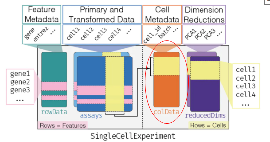
- 本质上为行名为sample的data.frame,即为细胞添加注释信息
如上,创建对象时,引入了sample的group分组信息
1
2
|
colData(sce) %>% head()
table(sce$group)
|
2.1 新增colData#
$符可用于查看colData,也能用于新增。(这一点等同于dataframe)
1
2
|
sce$anything <- runif(ncol(sce))
colnames(colData(sce))
|
1
2
|
sce <- scater::addPerCellQC(sce)
colData(sce)[, 1:5]
|
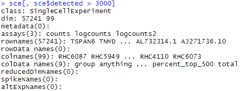
2.2 筛选sample#
1
2
|
sce[, sce$detected > 3000]
sce  #原来是160个sample
|
3、rowData结构#

参考colData,本质上为行名为feature的data.frame,即为基因添加注释信息。
- 可以在创建对象时添加(基因的不同ID),或者利用scater包添加注释。
1
|
sce <- scater::addPerFeatureQC(sce)
|
1
2
|
rowData(x) <- cbind(rowData(x), feature)
#同理colData也类似,但使用$符也很方便
|
1
2
|
sce[rownames(nm_count)[c(1:10)], ]
sce[1:10, ]
|
Furthermore, there is a special rowRanges slot to hold genomic coordinates in the form of a GRanges or GRangesList. This stores describes the chromosome, start, and end coordinates of the features (genes, genomic regions) in a manner that is easy to query and manipulate via the GenomicRanges framework.
4、reducedDims#

- 上面三点基本源于SummarizedExperiment对象,但reducedDims是sce对象独有的一点,一般储存PCA,tSNE,uMAP等细胞降维聚类信息;
- 本质是行名为sample的一组data.frame
1
2
3
4
5
6
7
8
9
|
sce <- scater::logNormCounts(sce)
sce <- scater::runPCA(sce)
reducedDim(sce, "PCA")
reducedDim(sce, "PCA")[1:4,1:4]
#           PC1    PC2     PC3   PC4
#RHC4104  46.66 -46.44  -9.488  1.79
#RHC6087 -54.38  -6.15  -0.155 13.16
#RHL2880  -7.89 -38.89  -1.319 -2.90
#RHC5949 -53.27 -20.88 -12.089 -7.73
|
1
2
3
4
5
6
7
8
|
sce <- scater::runTSNE(sce, perplexity = 0.1)
reducedDim(sce, "TSNE")  #可用于绘图的二维坐标信息
reducedDims(sce) #类比assays

u <- uwot::umap(t(logcounts(sce)), n_neighbors = 2)
reducedDim(sce, "UMAP_uwot") <- u
reducedDims(sce) # Now stored in the object.
reducedDim(sce, "UMAP_uwot") #可用于绘图的二维坐标信息
|