当分析多个样本的单细胞数据集时,其中重要的一步是判断并校正潜在的批次效应。如下简单学习两种单细胞批次效应分析方法,分别基于Seurat与harmony包。
1、示例数据#
- 来自Seurat提供的包含两个不同处理方式样本的单细胞表达矩阵。
 1
 2
 3
 4
 5
 6
 7
 8
 9
10
11
12
13
14
15
16
17
18
19
20
21
22
23
24
25
26
27
28
29
30
31
|
library(SeuratData)
InstallData("ifnb")
ifnb
# An object of class Seurat
# 14053 features across 13999 samples within 1 assay
# Active assay: RNA (14053 features, 0 variable features)
table(ifnb$stim) # CTRL与STIM两个样本
# CTRL STIM
# 6548 7451
table(ifnb$seurat_annotations) # 已注释细胞类型
# CD14 Mono CD4 Naive T CD4 Memory T CD16 Mono B CD8 T T activated
# 4362 2504 1762 1044 978 814 633
# NK DC B Activated Mk pDC Eryth
# 619 472 388 236 132
ifnb = ifnb %>%
NormalizeData() %>%
FindVariableFeatures() %>%
ScaleData() %>%
RunPCA(npcs = 30) %>%
RunUMAP(reduction = "pca", dims = 1:30)
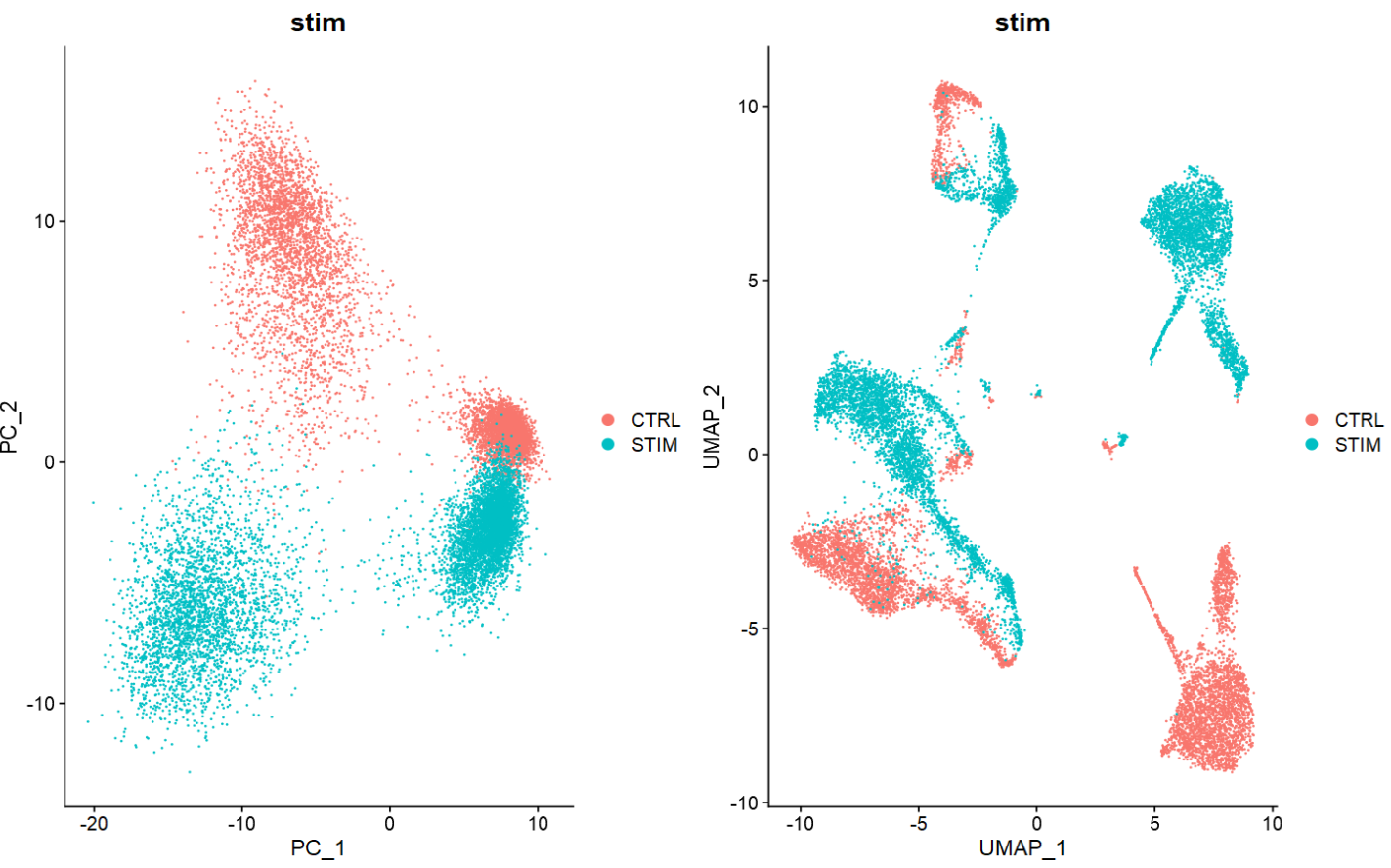
## 如下降维图,两个样本间存在较为明显的批次效应
p1 = DimPlot(ifnb,
reduction = "pca",
group.by = "stim")
p2 = DimPlot(ifnb,
reduction = "umap",
group.by = "stim")
p1 + p2
|
2、Seurat包分析#
参考教程:https://satijalab.org/seurat/articles/integration_rpca.html
 1
 2
 3
 4
 5
 6
 7
 8
 9
10
11
12
13
14
15
16
17
18
19
20
|
ifnb.list <- SplitObject(ifnb, split.by = "stim")
length(ifnb.list)
# [1] 2

##(1)标准化,鉴定高变基因
ifnb.list <- lapply(X = ifnb.list, FUN = function(x) {
  x <- NormalizeData(x)
  x <- FindVariableFeatures(x, selection.method = "vst", nfeatures = 2000)
})

##(2)鉴定共同的高变基因
features <- SelectIntegrationFeatures(object.list = ifnb.list)
str(features)
# chr [1:2000] "HBB" "HBA2" "HBA1" "CCL4" "CCL3" "CCL7" "TXN" "GNLY" "PPBP" "APOBEC3B" ...

##(3)归一化,降维
ifnb.list <- lapply(X = ifnb.list, FUN = function(x) {
  x <- ScaleData(x, features = features)
  x <- RunPCA(x, features = features)
})
|
- 对不同批次的Seurat对象进行校正:首先需要鉴定批次间锚点(Anchor),然后根据锚点合并样本。
- 其中,有若干种鉴定锚点的方法可供选择,分别是CCA与RPCA
- CCA方法:适合样本间细胞类型组成相同,且由于疾病状态或者其它明显影响因素造成较大的批次效应。缺点是容易过度校正,多样本分析比较慢。
- RPCA方法:适合样本细胞类型组成有些许差异,且对于多样本处理较快。
1
2
3
4
5
6
7
8
|
## (1) 鉴定锚点
anchors <- FindIntegrationAnchors(object.list = ifnb.list,
                                  anchor.features = features,
                                  reduction = "rpca")  # "cca"
## (2) 合并样本
combined <- IntegrateData(anchorset = anchors)
Assays(combined)
# [1] "RNA"        "integrated"
|
 1
 2
 3
 4
 5
 6
 7
 8
 9
10
11
12
13
14
15
|
DefaultAssay(combined) <- "integrated"
combined <- combined %>%
ScaleData(verbose = FALSE) %>%
RunPCA(npcs = 30) %>%
RunUMAP(reduction = "pca", dims = 1:30)
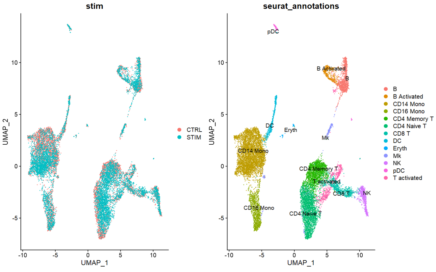
p1 <- DimPlot(combined,
reduction = "umap",
group.by = "stim")
p2 <- DimPlot(combined,
reduction = "umap",
group.by = "seurat_annotations",
label = TRUE,
repel = TRUE)
p1 + p2
|
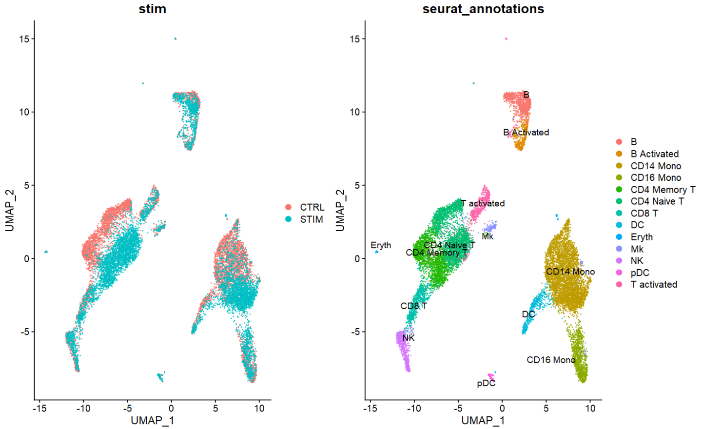
- 如上图,两个样本间大部分细胞类型得到较好的批次校正。但仍有例如CD4 naive/memory有较明显的分离。
- k.anchor是
FindIntegrationAnchors()的参数之一:值越大(默认为5),校正批次的力度越大。如下图是k.anchor设置为20的结果。
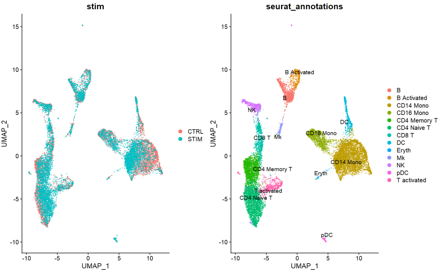
- 如下图是使用CCA鉴定锚点的分析结果,相比RPCA的校正结果更加显著。
- 在单样本数据预处理时,使用SCTransform代替。
 1
 2
 3
 4
 5
 6
 7
 8
 9
10
11
12
13
14
|
ifnb.list <- SplitObject(ifnb, split.by = "stim")
ifnb.list <- lapply(X = ifnb.list, FUN = SCTransform, method = "glmGamPoi")
features <- SelectIntegrationFeatures(object.list = ifnb.list,
                                      nfeatures = 3000)
ifnb.list <- PrepSCTIntegration(object.list = ifnb.list,
                                anchor.features = features)
ifnb.list <- lapply(X = ifnb.list, FUN = RunPCA, features = features)
anchors <- FindIntegrationAnchors(object.list = ifnb.list,
                                  normalization.method = "SCT",
                                  anchor.features = features,
                                  dims = 1:30, reduction = "rpca")
combined.sct <- IntegrateData(anchorset = anchors,
                              normalization.method = "SCT",
                              dims = 1:30)
|
3、harmony分析方法#
参考教程:https://portals.broadinstitute.org/harmony/articles/quickstart.html
harmony是2019年broad团队与Nature Method提出的单细胞样本间批次校正方法,其使用方法可以接入Seurat分析流程,简单方便。
 1
 2
 3
 4
 5
 6
 7
 8
 9
10
11
12
13
14
15
16
17
18
19
20
|
# 如第一步,已进行标准化等预处理
ifnb = ifnb %>%
RunHarmony("stim")
Reductions(ifnb)
# [1] "pca" "umap" "harmony"
Embeddings(ifnb, reduction = "harmony") %>% dim()
# [1] 13999 30
Embeddings(ifnb, reduction = "harmony")[,1:5] %>% head
# harmony_1 harmony_2 harmony_3 harmony_4 harmony_5
# AAACATACATTTCC.1 -11.5422398 0.9451146 1.8254414 -0.05006501 0.3120439
# AAACATACCAGAAA.1 -12.0970756 2.4677964 -2.7228544 -0.41740645 -1.6086122
# AAACATACCTCGCT.1 -9.6903638 2.5644996 -0.3257312 -0.85160456 0.4860005
# AAACATACCTGGTA.1 0.8948379 -1.9789529 13.4008741 5.95973200 -1.2721535
# AAACATACGATGAA.1 7.1235140 0.1124901 -1.4078848 -2.58582259 -0.1778708
# AAACATACGGCATT.1 -9.3618540 3.1966899 -3.1654761 -0.89614903 -0.1466429
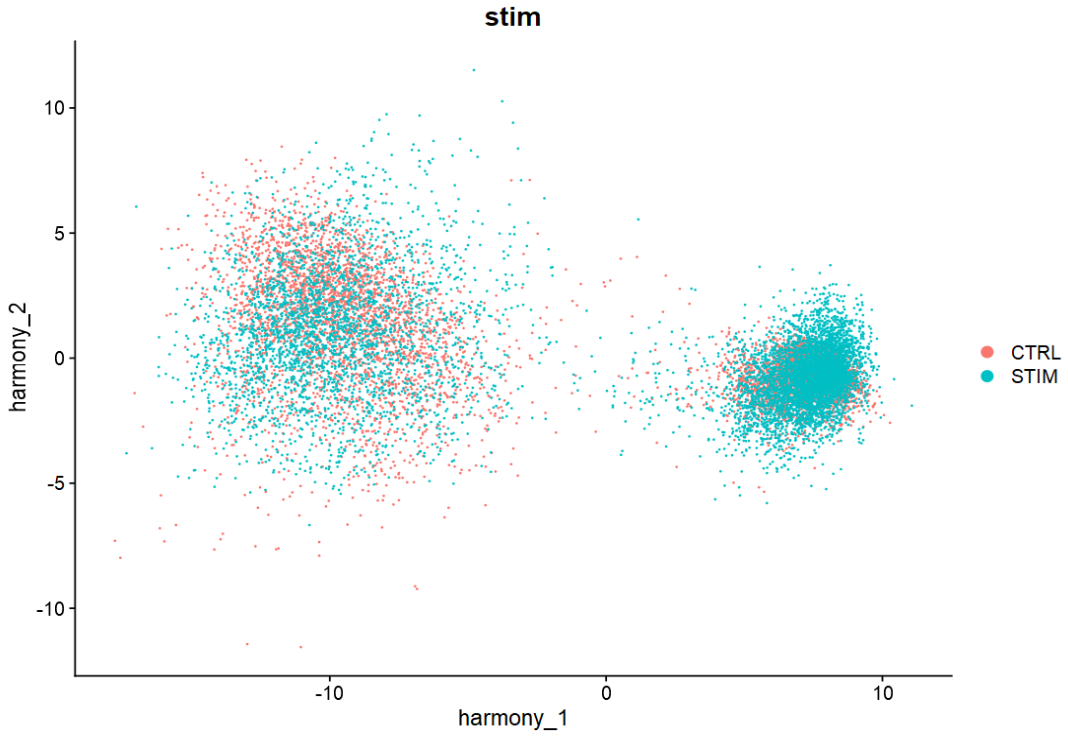
DimPlot(ifnb2,
reduction = "harmony",
group.by = "stim")
|