A cell cycle is a series of events that takes place in a cell as it grows and divides.即描述细胞生长、分裂整个过程中细胞变化过程。最重要的两个特点就是DNA复制、分裂成两个一样的子细胞。对于单细胞转录组数据,可根据相关marker基因的表达水平判断每一个细胞所处的细胞周期状态。此外在分析多数据集间批次效应时,可根据每个数据集中各个细胞周期比例进行判断与校正。
一、细胞周期阶段#
细胞周期相关基础知识具体可参考如下链接:
https://teachmephysiology.com/biochemistry/cell-growth-death/cell-cycle/
https://www.genome.gov/genetics-glossary/Cell-Cycle
细胞周期 _ 搜索结果_哔哩哔哩_Bilibili
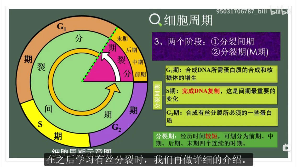
简单来说,一般可分成4个阶段
- G1(gap1):Cell increases in size(Cellular contents duplicated)
- S(synthesis) :DNA replication, each of the 46 chromosomes (23 pairs) is replicated by the cell
- G2(gap2):Cell grows more,organelles and proteins develop in preparation for cell division
- M(mitosis):‘Old’ cell partitions the two copies of the genetic material into the two daughter cells. And the cell cycle can begin again.
在处理单细胞数据时,分析细胞周期可对于生物机制探索或者潜在批次效应判断提供另一种角度的见解。由于细胞周期也是通过cell cycle related protein 调控,即每个阶段有显著的marker基因;通过分析细胞周期有关基因的表达情况,可以对细胞所处周期阶段进行注释。
Note:在单细胞周期分析时,通常只考虑三个阶段:G1、S、G2M。(即把G2和M当做一个phase)
如下简单学习分析单细胞细胞周期的两种方法,示例数据集来自10X的PBMC样本
 1
 2
 3
 4
 5
 6
 7
 8
 9
10
11
12
13
14
15
|
library(Seurat)
library(tidyverse)
# download.file("https://cf.10xgenomics.com/samples/cell-exp/1.1.0/pbmc3k/pbmc3k_filtered_gene_bc_matrices.tar.gz",
# "pbmc3k_filtered_gene_bc_matrices.tar.gz")
# untar("pbmc3k_filtered_gene_bc_matrices.tar.gz")
pbmc.data = Read10X(data.dir = "filtered_gene_bc_matrices/hg19/")
pbmc = CreateSeuratObject(counts = pbmc.data, project = "pbmc3k")
pbmc = NormalizeData(pbmc) %>%
FindVariableFeatures()
pbmc = ScaleData(pbmc) %>%
RunPCA() %>%
RunUMAP(dims = 1:30)
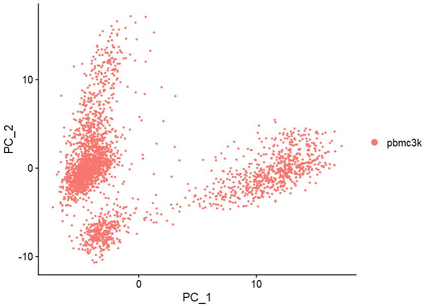
DimPlot(pbmc, reduction = "pca")
|
二、Seurat包分析#
- Seurat包细胞周期分析的基本原理类似模块打分。
- 首先该包定义了S期与G2M期的基因模块,分别对每个单细胞进行打分。
- 若S期基因模块分数高,则认为细胞处于S期;同理分析G2M期。若二者分数均较低,则认为是G1期。
 1
 2
 3
 4
 5
 6
 7
 8
 9
10
11
12
13
14
15
16
17
18
19
20
|
str(cc.genes)
# List of 2
# $ s.genes : chr [1:43] "MCM5" "PCNA" "TYMS" "FEN1" ...
# $ g2m.genes: chr [1:54] "HMGB2" "CDK1" "NUSAP1" "UBE2C" ...
## CellCycleScoring()函数分析细胞周期
pbmc = CellCycleScoring(pbmc,
s.features = cc.genes$s.genes,
g2m.features = cc.genes$g2m.genes)
head(pbmc@meta.data[,c("S.Score", "G2M.Score", "Phase")])
# S.Score G2M.Score Phase
# AAACATACAACCAC-1 0.07721641 -0.027546191 S
# AAACATTGAGCTAC-1 -0.02723808 -0.038481308 G1
# AAACATTGATCAGC-1 -0.01832618 0.069915003 G2M
# AAACCGTGCTTCCG-1 0.01548134 0.008207127 S
# AAACCGTGTATGCG-1 -0.05922341 0.031726222 G2M
# AAACGCACTGGTAC-1 -0.05420895 -0.063251247 G1
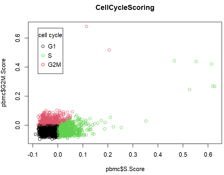
table(pbmc$Phase)
# G1 G2M S
# 1437 544 719
|
1
2
3
4
5
6
7
8
|
plot(pbmc$S.Score,
     pbmc$G2M.Score,
     col=factor(pbmc$Phase),
     main="CellCycleScoring")
legend("topleft", inset=0.05,
       title = "cell cycle",
       c("G1","S","G2M"),
       pch = c(1), col=c("black","green","red"))
|
1
2
|
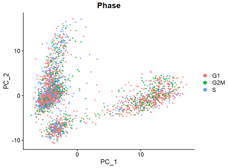
DimPlot(pbmc, reduction = "pca",
        group.by = "Phase")
|
Seurat包提供的cc.genes为人类基因名。如果需分析小鼠数据,可将其转换为鼠源基因名。
 1
 2
 3
 4
 5
 6
 7
 8
 9
10
11
12
13
14
15
|
## 人工转换(考验网络)
convertHumanGeneList <- function(x){
  require("biomaRt")
  human = useMart("ensembl", dataset = "hsapiens_gene_ensembl")
  mouse = useMart("ensembl", dataset = "mmusculus_gene_ensembl")
  genesV2 = getLDS(attributes = c("hgnc_symbol"), filters = "hgnc_symbol", values = x , mart = human, attributesL = c("mgi_symbol"), martL = mouse, uniqueRows=T)
  humanx <- unique(genesV2[, 2])
  print(head(humanx))
  return(humanx)
}
m.s.genes <- convertHumanGeneList(cc.genes$s.genes)
m.g2m.genes <- convertHumanGeneList(cc.genes$g2m.genes)

## github下载
# https://github.com/satijalab/seurat/issues/462
|
三、scran包分析#
- scran包细胞周期分析的基本原理是 gene pair表达特征比较
- 首先该包分别提供了三种细胞周期的gene pair表达特征,其中first列表达水平均高于second列。
- 然后分析每个单细胞的相应gene pair表达水平,比较最符合哪一类细胞周期的特征。
 1
 2
 3
 4
 5
 6
 7
 8
 9
10
11
12
13
|
library(scran)
hs.pairs = readRDS(system.file("exdata", "human_cycle_markers.rds", package="scran"))
# mm.pairs = readRDS(system.file("exdata", "mouse_cycle_markers.rds", package="scran"))
names(hs.pairs)
# [1] "G1"  "S"   "G2M"
head(hs.pairs$G2M)
#             first          second
# 1 ENSG00000100519 ENSG00000065135
# 2 ENSG00000100519 ENSG00000080345
# 3 ENSG00000100519 ENSG00000151914
# 4 ENSG00000100519 ENSG00000085224
# 5 ENSG00000100519 ENSG00000116133
# 6 ENSG00000100519 ENSG00000143924
|
如上示意,特征数据的基因名为ENSEMBL的ID格式。可根据需要对单细胞表达矩阵的行名进行转换。
 1
 2
 3
 4
 5
 6
 7
 8
 9
10
11
12
13
14
15
16
17
18
19
20
21
22
23
24
25
|
mt_count = pbmc@assays$RNA@counts
mt_count[1:4,1:4]
# 4 x 4 sparse Matrix of class "dgCMatrix"
#              AAACATACAACCAC-1 AAACATTGAGCTAC-1 AAACATTGATCAGC-1 AAACCGTGCTTCCG-1
# MIR1302-10                  .                .                .                .
# FAM138A                     .                .                .                .
# OR4F5                       .                .                .                .
# RP11-34P13.7                .                .                .                .
str(rownames(mt_count))
# chr [1:32738] "MIR1302-10" "FAM138A" "OR4F5" "RP11-34P13.7" "RP11-34P13.8" ...

## ID转换
library(org.Hs.eg.db)
gene_ids = AnnotationDbi::select(org.Hs.eg.db,
                                 keys=rownames(mt_count),
                                 columns=c("ENSEMBL"),
                                 keytype="SYMBOL")
gene_ids = gene_ids %>%
  na.omit() %>%
  dplyr::distinct(SYMBOL, .keep_all = T) %>%
  dplyr::distinct(ENSEMBL, .keep_all = T)
mt_count = mt_count[gene_ids$SYMBOL,]
rownames(mt_count) = gene_ids$ENSEMBL
dim(mt_count)
# [1] 18893  2700
|
 1
 2
 3
 4
 5
 6
 7
 8
 9
10
11
12
13
14
|
assignments = scran::cyclone(mt_count,
                      pairs = hs.pairs)
names(assignments)
# [1] "phases"            "scores"            "normalized.scores"
dim(assignments$normalized.scores)
# [1] 2700    3
assignments$normalized.scores[1:3,]
#          G1         S         G2M
# 1 0.8118324 0.1865242 0.001643385
# 2 0.4174428 0.5427604 0.039796782
# 3 0.7157215 0.2842785 0.000000000
table(assignments$phases)
#   G1  G2M    S
# 2551   60   89
|
1
2
3
4
5
6
7
|
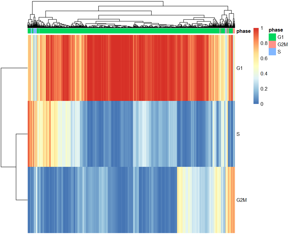
scores = t(assignments$scores)
colnames(scores)=1:ncol(scores)
library(pheatmap)
pheatmap(scores,
         show_colnames = F,
         annotation_col=data.frame(phase=assignments$phases,
                                   row.names = 1:ncol(scores)))
|
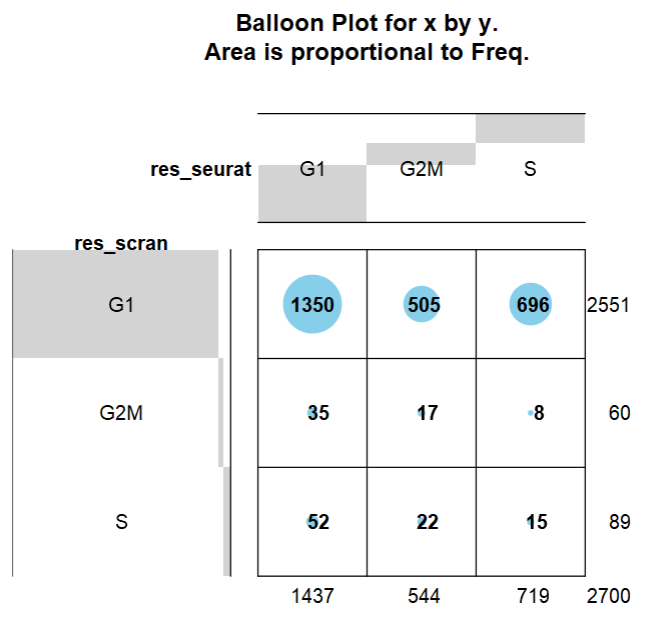
最后比较一下两种方法注释结果的差异
1
2
3
4
5
6
7
8
9
|
res_seurat = pbmc$Phase
res_scran = assignments$phases
tb = table(res_seurat, res_scran)
#           res_scran
# res_seurat   G1  G2M    S
#        G1  1350   35   52
#        G2M  505   17   22
#        S    696    8   15
gplots::balloonplot(tb)
|