WGCNA是适用于大批量样本的array或者Bulk RNAseq数据的加权基因共表达网络分析。由于单细胞数据的稀疏性,不适用于WGCNA直接分析。hdWGCNA包基于WGCNA包提供了一种针对scRNAseq数据的加权基因共表达网络分析策略。
官方教程:https://smorabit.github.io/hdWGCNA/articles/basic_tutorial.html
1、加载包并准备示例数据#
 1
 2
 3
 4
 5
 6
 7
 8
 9
10
11
12
13
|
#devtools::install_github('smorabit/hdWGCNA', ref='dev')
library(hdWGCNA)
library(WGCNA)

library(Seurat)
library(clustree)
library(dplyr)
library(patchwork)

# 示例数据
#  https://cf.10xgenomics.com/samples/cell/pbmc3k/pbmc3k_filtered_gene_bc_matrices.tar.gz
list.files("filtered_gene_bc_matrices/hg19/")
# [1] "barcodes.tsv" "genes.tsv"    "matrix.mtx"
|
2、创建Seurat对象并预处理#
执行Seurat的常规流程,包括:创建seurat对象—标准化、归一化—高变基因—降维、聚类分群—鉴定细胞类型(optional)
 1
 2
 3
 4
 5
 6
 7
 8
 9
10
11
12
13
14
15
16
17
18
19
20
|
sce = Read10X(data.dir = "filtered_gene_bc_matrices/hg19/") %>% CreateSeuratObject()
# 32738 features across 2700 samples

sce = sce %>%
  NormalizeData() %>%
  FindVariableFeatures() %>%
  ScaleData()
sce = sce %>%
  RunPCA() %>%
  RunUMAP(dims = 1:30) %>%  #RunTSNE
  FindNeighbors(dims = 1:30) %>%
  FindClusters(resolution = c(0.01, 0.05, 0.1, 0.2, 0.3, 0.5,0.8,1))

clustree(sce@meta.data, prefix = "RNA_snn_res.")
#colnames(sce@meta.data)
table(sce$RNA_snn_res.0.1)
#    0    1    2    3
# 1195  698  448  359
Idents(sce) = "RNA_snn_res.0.1"
##如上按照分辨率为0.1的分群结果进行后续的分析
|
3、创建misc slot,挑选基因#
 1
 2
 3
 4
 5
 6
 7
 8
 9
10
11
12
13
14
15
16
17
|
seurat_obj = SetupForWGCNA(
  sce,
  gene_select = "fraction", # the gene selection approach
  fraction = 0.05, # fraction of cells that a gene needs to be expressed in order to be included
  wgcna_name = "PBMC" # the name of the hdWGCNA experiment
)

# gene_select参数设置过滤基因的方法,还有是
## (1) "variable" :  use the genes stored in the Seurat object’s VariableFeatures.
## (2) "custom"   :  use genes that are specified in a custom list.

str(seurat_obj@misc)
# List of 2
#  $ active_wgcna: chr "PBMC"
#  $ PBMC        :List of 2
#   ..$ wgcna_group: chr "all"
#   ..$ wgcna_genes: chr [1:3855] "NOC2L" "HES4" "ISG15" "TNFRSF4" ...
|
将多个细胞表达情况(KNN)合并为一个metacell,可避免单细胞数据的稀疏性。
“多个细胞"需要是来自同一种细胞类型/分群,可通过group.by参数定义依据。
k参数:in general a lower number for k can be used for small datasets. We generally use k values between 20 and 75.
 1
 2
 3
 4
 5
 6
 7
 8
 9
10
11
12
13
14
15
16
17
18
19
20
21
22
23
24
25
26
|
seurat_obj <- MetacellsByGroups(
  seurat_obj = seurat_obj,
  group.by = c("RNA_snn_res.0.1"), # specify the columns in seurat_obj@meta.data to group by
  k = 25, # nearest-neighbors parameter
  max_shared = 10, # maximum number of shared cells between two metacells
  ident.group = 'RNA_snn_res.0.1' # set the Idents of the metacell seurat object
)
seurat_obj <- NormalizeMetacells(seurat_obj)

seurat_obj@misc$PBMC$wgcna_metacell_obj
# 32738 features across 1524 samples within 1 assay
seurat_obj@misc$PBMC$wgcna_metacell_obj@assays$RNA@counts[1:4,1:8]
# 4 x 8 sparse Matrix of class "dgCMatrix"
#              0_1 0_2 0_3 0_4 0_5 0_6 0_7 0_8
# MIR1302-10     .   .   .   .   .   .   .   .
# FAM138A        .   .   .   .   .   .   .   .
# OR4F5          .   .   .   .   .   .   .   .
# RP11-34P13.7   .   .   .   .   .   .   .   .
seurat_obj@misc$PBMC$wgcna_metacell_obj@meta.data %>% head
#     orig.ident nCount_RNA nFeature_RNA RNA_snn_res.0.1
# 0_1          0    2618.96         5880               0
# 0_2          0    2486.00         5858               0
# 0_3          0    1340.56         4306               0
# 0_4          0    2112.12         5388               0
# 0_5          0    2839.04         6073               0
# 0_6          0    2198.44         5407               0
|
5、共表达网络分析#
 1
 2
 3
 4
 5
 6
 7
 8
 9
10
11
12
13
14
15
16
|
##(1) 选择一种/多种细胞类型,进行WGCNA分析
seurat_obj <- SetDatExpr(
seurat_obj,
group_name = c(0,1,2,3),
group.by='RNA_snn_res.0.1' # the metadata column containing the cell type info. This same column should have also been used in MetacellsByGroups
)
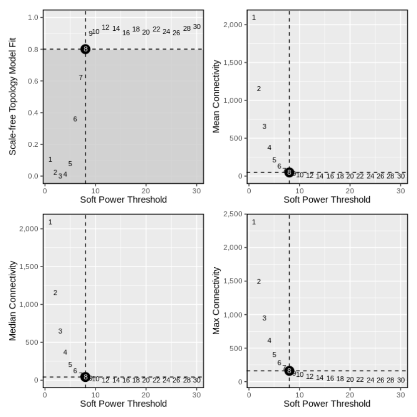
##(2) 选择合适的软阈值
seurat_obj <- TestSoftPowers(
seurat_obj,
setDatExpr = FALSE, # set this to FALSE since we did this above
)
plot_list <- PlotSoftPowers(seurat_obj)
wrap_plots(plot_list, ncol=2)
# power_table <- GetPowerTable(seurat_obj)
# head(power_table)
|
1
2
3
4
5
6
|
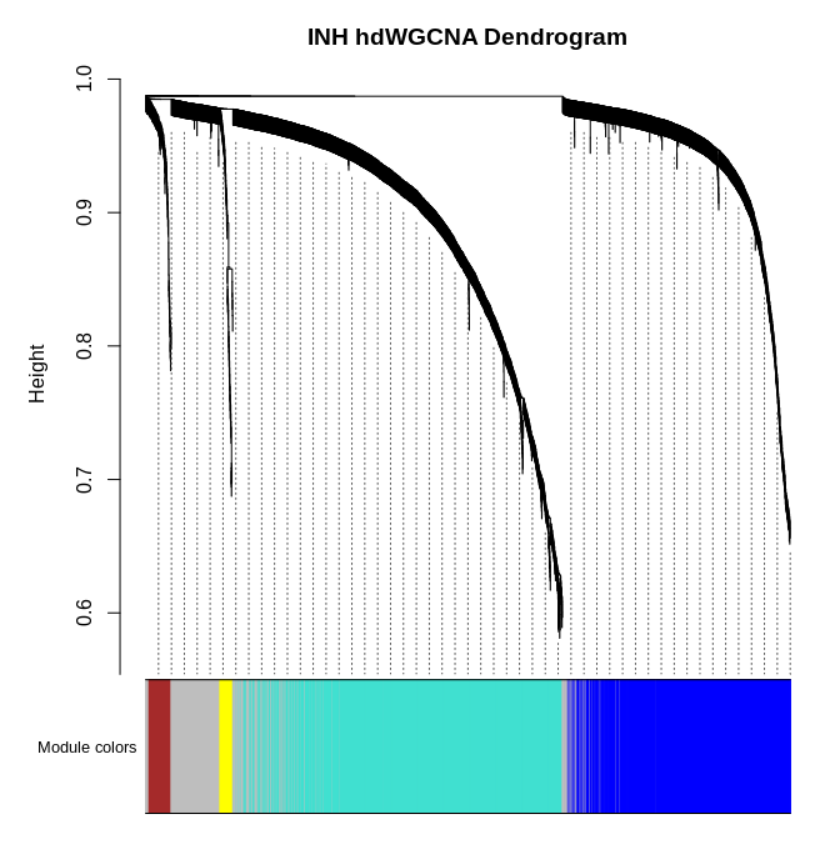
##(3) 根据上图选择合适的软阈值构建网络
seurat_obj <- ConstructNetwork(
  seurat_obj, soft_power=8,
  setDatExpr=FALSE
)
PlotDendrogram(seurat_obj, main='INH hdWGCNA Dendrogram')
|
6、模块特征值与hub基因分析#
 1
 2
 3
 4
 5
 6
 7
 8
 9
10
11
12
13
14
|
seurat_obj@misc$PBMC$wgcna_modules %>% head
#         gene_name    module     color
# NOC2L       NOC2L      grey      grey
# HES4         HES4 turquoise turquoise
# ISG15       ISG15 turquoise turquoise
# TNFRSF4   TNFRSF4      blue      blue
# SDF4         SDF4      blue      blue
# UBE2J2     UBE2J2      blue      blue

table(seurat_obj@misc$PBMC$wgcna_modules$module)
# grey turquoise      blue     brown    yellow
#  588      1786      1272       133        76
# modules <- GetModules(seurat_obj)
# head(modules)
|
 1
 2
 3
 4
 5
 6
 7
 8
 9
10
11
12
13
14
|
seurat_obj <- ModuleEigengenes(
 seurat_obj
)
seurat_obj@misc$PBMC$MEs %>% head
#                        blue       grey      brown turquoise     yellow
# AAACATACAACCAC-1   4.755930  0.2424180  2.6565029 -5.832575 -2.0906948
# AAACATTGAGCTAC-1   2.388492  1.3106515 -0.3341197  1.172415  8.8764667
# AAACATTGATCAGC-1   5.807490  2.9008702  0.8873175 -1.132285 -1.8973713
# AAACCGTGCTTCCG-1  -6.662387 -0.3072945 -1.5451723 14.692779  0.1159869
# AAACCGTGTATGCG-1 -16.098322 -1.6676024  8.7666564 -4.131657 -0.9371790
# AAACGCACTGGTAC-1   2.064300 -0.1415680 -1.2313300 -2.824847 -1.1698044

# MEs <- GetMEs(seurat_obj, harmonized=FALSE)
# head(MEs)
|
- (3)鉴定模块内hub基因– 基因表达与模块特征值的具有高相关性
 1
 2
 3
 4
 5
 6
 7
 8
 9
10
11
12
13
14
15
16
17
18
19
20
21
22
23
24
25
26
27
28
29
30
31
32
33
34
35
36
37
38
39
40
41
42
43
44
45
46
47
48
49
50
|
seurat_obj <- ModuleConnectivity(
  seurat_obj
)
seurat_obj@misc$PBMC$wgcna_modules[,c(-1,-2,-3)] %>% head
#            kME_blue   kME_grey   kME_brown kME_turquoise   kME_yellow
# NOC2L    0.02851618 0.08360662  0.02041163   0.003048238  0.038497122
# HES4    -0.24225802 0.06869209 -0.08284058   0.117744840  0.326692215
# ISG15   -0.29705821 0.08027215 -0.07240235   0.351103776  0.314836382
# TNFRSF4  0.16100218 0.08589770  0.13010946  -0.002353201 -0.090182722
# SDF4     0.01120696 0.13914234  0.07918151   0.040070556  0.003869467
# UBE2J2   0.03178884 0.07651548  0.04663831   0.008615164 -0.006942615

# p <- PlotKMEs(seurat_obj, ncol=2)
# p

hub_df <- GetHubGenes(seurat_obj, n_hubs = 10)
hub_df
#   gene_name    module       kME
# 1     RPS27      blue 0.7207118
# 2     RPS12      blue 0.7258250
# 3      CCL5     brown 0.4934812
# 4       B2M     brown 0.5294537
# 5    LGALS1 turquoise 0.6477877
# 6    TYROBP turquoise 0.6542149
# 7   HLA-DRA    yellow 0.5817169
# 8  HLA-DPA1    yellow 0.5894472

## 计算每个细胞对于每个模块hub基因的表达活性(module score),可使用seurat包或者Ucell包
seurat_obj <- ModuleExprScore(
  seurat_obj,
  n_genes = 25,
  method='Seurat'
)
seurat_obj@misc$PBMC$module_scores %>% head
## 计算每个细胞对于每个模块hub基因的表达活性(module score),可使用seurat包或者Ucell包
#                      blue      brown turquoise      yellow
# AAACATACAACCAC-1 3.380281 0.74403040 0.3806462 -0.18699177
# AAACATTGAGCTAC-1 3.035111 0.31949694 0.4019337  1.06061130
# AAACATTGATCAGC-1 2.769994 0.28652286 0.5089602 -0.30358276
# AAACCGTGCTTCCG-1 2.080403 0.07190668 2.6016017  0.45921797
# AAACCGTGTATGCG-1 1.434566 1.07243443 0.9849420  0.14309843
# AAACGCACTGGTAC-1 2.999822 0.25594526 0.6041499 -0.02860217

# library(UCell)
# seurat_obj <- ModuleExprScore(
#   seurat_obj,
#   n_genes = 25,
#   method='UCell'
# )
# seurat_obj@misc$PBMC$module_scores %>% head
|
7、结果可视化#
1
2
3
4
5
6
|
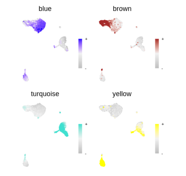
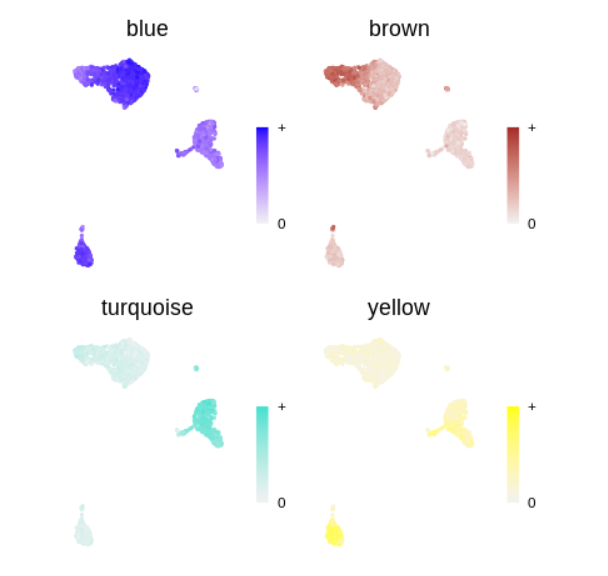
plot_list <- ModuleFeaturePlot(
  seurat_obj,
  features='MEs', # plot the hMEs
  order=TRUE # order so the points with highest hMEs are on top
)
wrap_plots(plot_list, ncol=2)
|
1
2
3
4
5
6
7
8
|
seurat_obj@misc$PBMC$module_scores %>% head
plot_list <- ModuleFeaturePlot(
  seurat_obj,
  features='scores', # plot the hub gene scores
  order='shuffle', # order so cells are shuffled
  ucell = TRUE # depending on Seurat vs UCell for gene scoring
)
wrap_plots(plot_list, ncol=2)
|
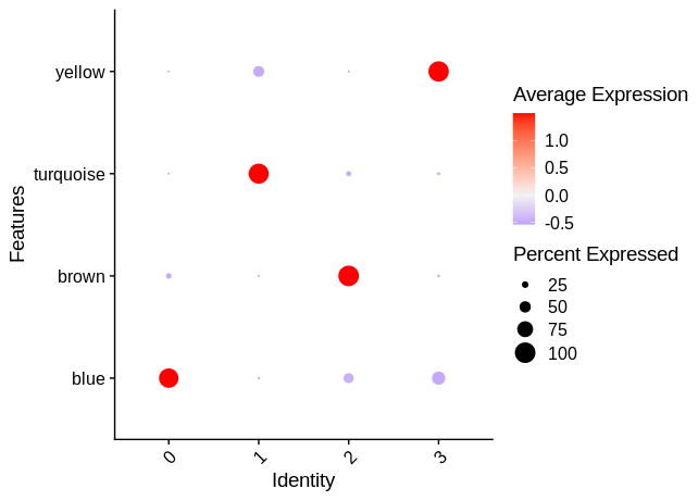
- 将细胞对于模块的特征值,整合到seurat的meta.data中
 1
 2
 3
 4
 5
 6
 7
 8
 9
10
|
MEs <- GetMEs(seurat_obj)
mods <- colnames(MEs); mods <- mods[mods != 'grey']
seurat_obj@meta.data <- cbind(seurat_obj@meta.data, MEs)

p <- DotPlot(seurat_obj, features = mods, group.by = 'RNA_snn_res.0.1')
p <- p +
  coord_flip() +
  RotatedAxis() +
  scale_color_gradient2(high='red', mid='grey95', low='blue')
p
|