单细胞数据分析常用的Seurat包也集成了空间转录组的分析流程。
https://satijalab.org/seurat/articles/spatial_vignette.html。
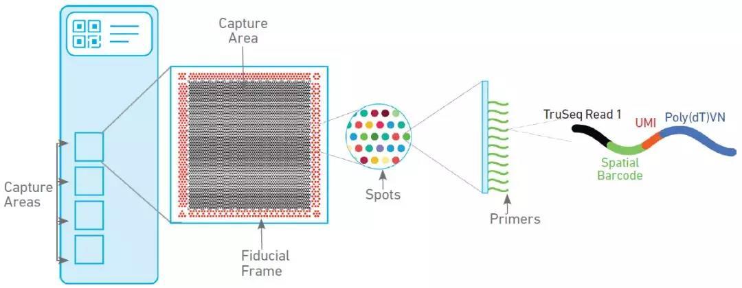
空间转录组可以简单理解为在2D组织切面的多个采样spot进行测序,同时记录下每个spot在切片中的2维坐标位置。
在Seurat流程数据分析时可以将一个spot视为一个细胞(实际上还没有达到单细胞分辨率),然后基本可按照一般单细胞数据分析流程。
0、数据准备#
来自10X官方提供的小鼠脑部空间转录组测序数据,分为anterior与posterior两个切片。
以其中一张切片所包含的数据为例,可分为两部分数据。
(1)每个spot的基因表达测序数据,基本类似单细胞测序结果格式可以是三元组或者h5格式等
1
2
3
4
5
6
7
8
|
list.files("posterior/", recursive = TRUE)
# [1] "filtered_feature_bc_matrix.h5"
# [2] "filtered_feature_bc_matrix/barcodes.tsv.gz"
# [3] "filtered_feature_bc_matrix/features.tsv.gz"
# [4] "filtered_feature_bc_matrix/matrix.mtx.gz"
# [5] "spatial/scalefactors_json.json"
# [6] "spatial/tissue_lowres_image.png"
# [7] "spatial/tissue_positions_list.csv"
|
(2)每个spot在组织切片中的位置信息
- 首先是组织切片图片(tissue_lowres_image.png),需要查看确认一下图片的分辨率。如下示例图片为600×600
- 然后是每个spot在实际测序过程中的位置信息。(tissue_positions_list.csv)
- 第一列:spot的名字,对应于测序数据的spot ID
- 第二列:1/0,表示是否为组织测序区域
- 第三、四列:每个spot的相对位置坐标
- 第五、六列:每个spot在组织图片中的绝对位置(像素单位)
1
2
3
4
5
6
7
|
spot_meta = read.csv("posterior/spatial/tissue_positions_list.csv",
                     header = FALSE)
head(spot_meta)    #tissue row col imagerow imagecol
#                   V1 V2 V3 V4   V5   V6
# 1 ACGCCTGACACGCGCT-1  0  0  0 1419 1432
# 2 TACCGATCCAACACTT-1  0  1  1 1538 1501
# 3 ATTAAAGCGGACGAGC-1  0  0  2 1419 1570
|
- 最后是一个json文件(scalefactors_json.json),用于记录tissue_positions_list.csv所记录的spot绝对坐标与tissue_lowres_image.png图片的比例关系。以及spot的直径大小。
- 例如 (1419, 1432)*0.0516=(73.2204, 73.8912)即为在tissue_lowres_image.png中的坐标位置。
1
2
3
4
|
{
"fiducial_diameter_fullres": 144.59793566029023,
"tissue_lowres_scalef": 0.051635113
}
|
https://github.com/satijalab/seurat/issues/4993
There are four scaling factors that 10X provides, but we generally only use the lowres factor. If you’re using your own, non-10X data, simply create a fake scalefactors object with scalefactors, making sure that you use the correct factor for lowres. If you coordinates match 1:1 with your image, then your lowres scale factor would be 1
1、创建Seurat对象#
思路:先根据spot基因表达数据创建Seurat对象,然后加入组织图片以及spot的位置信息。
1.1 分步创建#
 1
 2
 3
 4
 5
 6
 7
 8
 9
10
11
12
13
14
15
16
17
18
19
20
21
22
23
24
25
26
27
28
29
30
31
32
33
34
35
36
37
38
39
40
|
##(1)构建传统seurat对象
sce = Read10X("posterior/filtered_feature_bc_matrix/") %>%
  CreateSeuratObject(assay = "Spot")     #将assay名设置为Spatial
# sce <- Read10X_h5("posterior/filtered_feature_bc_matrix.h5") %>%
#   CreateSeuratObject(assay = "Spatial")
dim(sce)
# [1] 32285  3355
# 3355个spot的32285个基因的表达
sce@assays$Spot@counts[1:4,1:4]
# 4 x 4 sparse Matrix of class "dgCMatrix"
#         AAACAAGTATCTCCCA-1 AAACACCAATAACTGC-1 AAACAGAGCGACTCCT-1 AAACAGCTTTCAGAAG-1
# Xkr4                     .                  .                  .                  .
# Gm1992                   .                  .                  .                  .
# Gm19938                  .                  1                  .                  .
# Gm37381                  .                  .                  .                  .
head(sce@meta.data)
#                       orig.ident nCount_Spot nFeature_Spot
# AAACAAGTATCTCCCA-1 SeuratProject        9195          3089
# AAACACCAATAACTGC-1 SeuratProject       33655          6468
# AAACAGAGCGACTCCT-1 SeuratProject       19619          5245

##(2)加入image信息
image <- Read10X_Image(image.dir = "posterior/spatial/")
image@image %>% dim()
# [1] 600 600   3
#image <- image[Cells(x = sce)]
image@coordinates %>% head()
#                    tissue row col imagerow imagecol
# TGGGACCATTGGGAGT-1      1   7   5     2257     1776
# CCGGTGCGAGTGATAG-1      1   7   7     2257     1914
# TAGCCAGAGGGTCCGG-1      1   7   9     2257     2052
image@scale.factors  #储存json信息
DefaultAssay(image) <- "Spot"
DefaultAssay(image)
sce[["posterior"]] <- image
sce
# An object of class Seurat
# 32285 features across 3355 samples within 1 assay
# Active assay: Spot (32285 features, 0 variable features)
# 1 image present: posterior
|
1.2 一步创建#
Load10X_Spatial()函数支持在准备好相应的文件基础上,一步创建出包含image信息的seurat对象
-
测序表达数据的h5文件
1
|
# [1] "filtered_feature_bc_matrix.h5"
|
-
图片及位置信息的spatial文件夹
1
2
|
list.files("posterior/spatial/")
# [1] "scalefactors_json.json"    "tissue_lowres_image.png"   "tissue_positions_list.csv"
|
1
2
3
4
5
|
sce = Load10X_Spatial(data.dir = "./posterior/",slice = "posterior")
# An object of class Seurat
# 32285 features across 3355 samples within 1 assay
# Active assay: Spatial (32285 features, 0 variable features)
# 1 image present: posterior
|
2、分析流程与可视化#
之后的分析可基本参考Seurat单细胞数据分析流程,完成spot的过滤、标准化、聚类分群、差异分析等;就不过多介绍了。
主要会在可视化方面有空间转录组自身独特的展示方式。
2.1 常规分析流程#
 1
 2
 3
 4
 5
 6
 7
 8
 9
10
11
12
13
14
15
16
17
18
|
##标准化
sce <- SCTransform(sce,assay = "Spot")

##降维
sce <- RunPCA(sce)
sce <- RunUMAP(sce, dims = 1:30, label = T)

##聚类分群
sce <- FindNeighbors(sce,dims = 1:20)
sce <- FindClusters(sce,resolution = 0.1)
table(sce$seurat_clusters)
#    0    1    2    3    4    5    6
# 1161  659  483  396  235  230  191

##差异分析
dif <- FindAllMarkers(sce, assay = "Spot", only.pos = T)
sig.dif <- dif%>%group_by(cluster) %>% top_n(n = 5,wt = avg_log2FC)
genes <- unique(sig.dif$gene)
|
2.2 可视化#
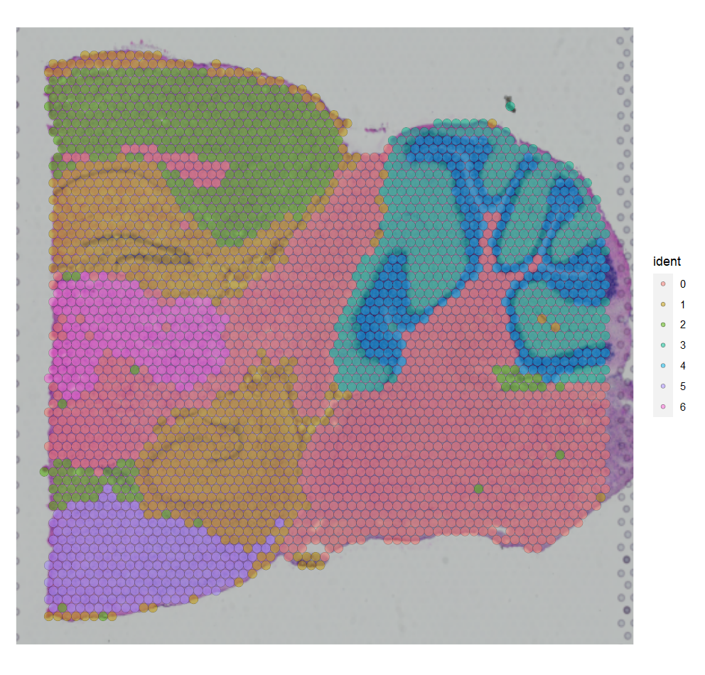
这里主要记录空间转录组自身独特的展示方式:以测序组织图片为背景,展示spot的聚类信息或者特定基因在每个spot的表达信息。
1
2
3
4
5
6
7
|
SpatialDimPlot(sce, alpha = 0.5)
SpatialDimPlot(sce,
               cells.highlight = CellsByIdentities(sce,idents = "1"))
SpatialDimPlot(sce,cells.highlight = CellsByIdentities(sce,idents = c("0","2")),
               facet.highlight = T)
SpatialDimPlot(sce,cells.highlight = CellsByIdentities(sce,idents = c("0","2","3")),
               facet.highlight = T)
|
1
|
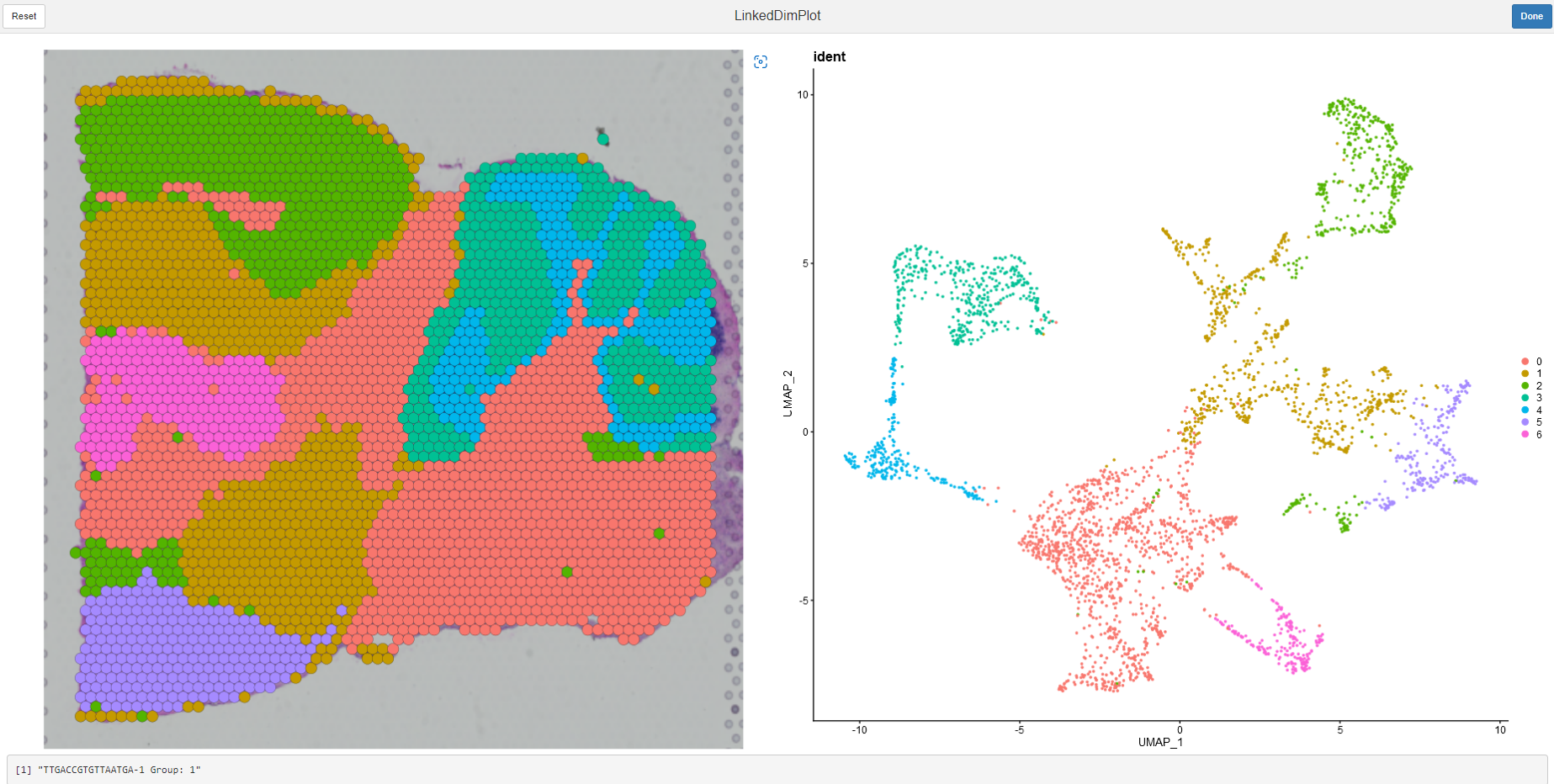
LinkedDimPlot(sce,reduction = "umap")
|
1
2
|
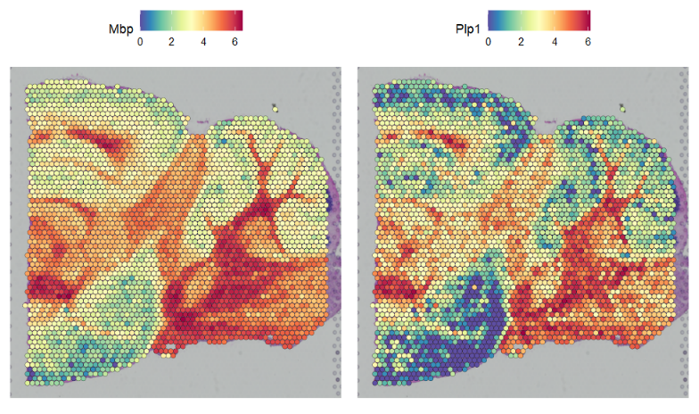
SpatialFeaturePlot(sce,features = genes[1:2],interactive = F)
SpatialFeaturePlot(sce,features = genes[1],pt.size=1.5,alpha=c(0.1,1),interactive = T)
|
1
|
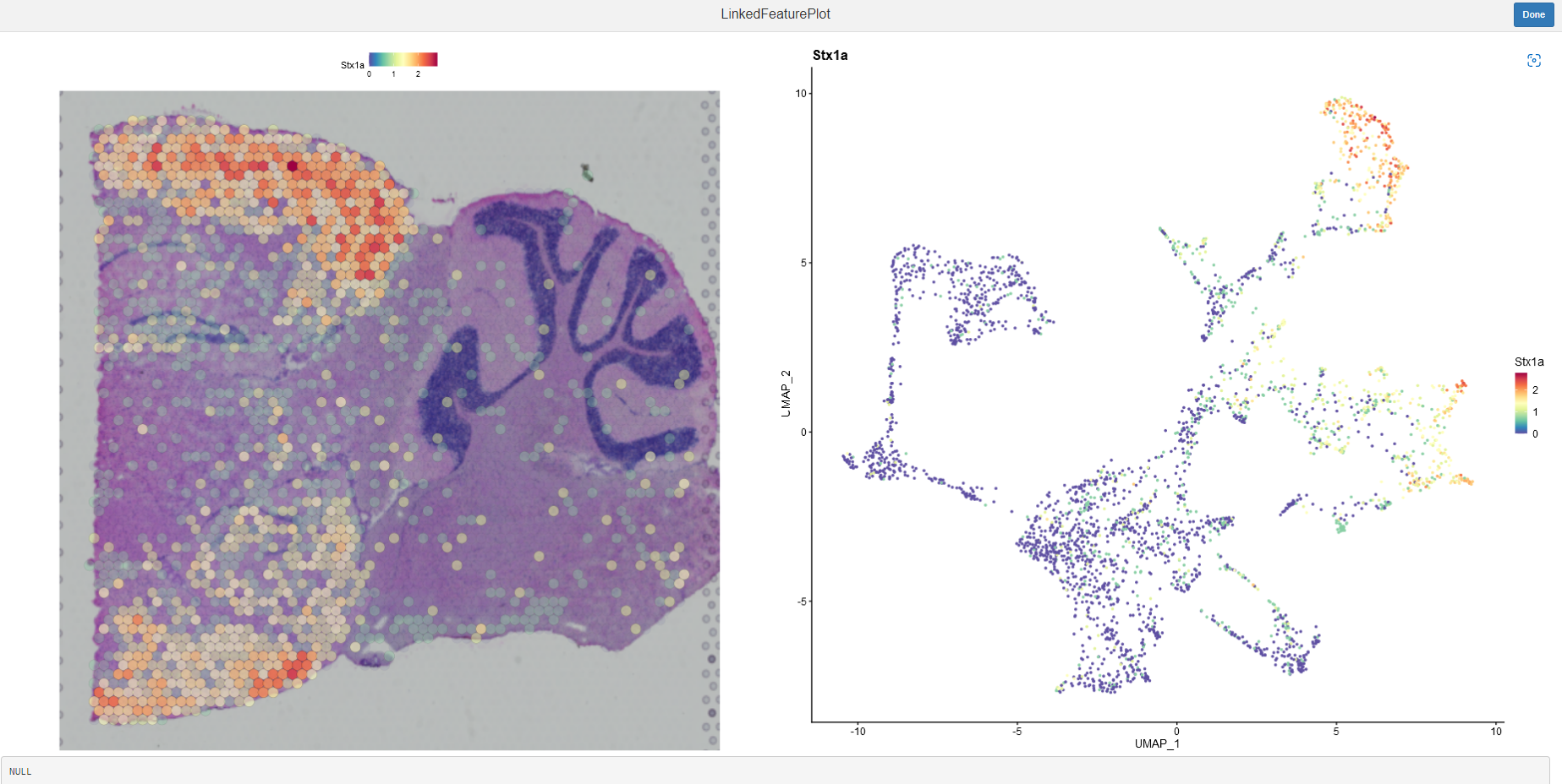
LinkedFeaturePlot(sce, feature = "Stx1a")
|
3、合并多个切片分析#
类似合并多个单细胞测序样本分析,此时每个Seurat对象都要有自己的image信息。必要时也可以使用批次校正等工具。
 1
 2
 3
 4
 5
 6
 7
 8
 9
10
11
|
anterior1 <- Load10X_Spatial(data.dir = "./Anterior",slice = "anterior")
posterior1 <- Load10X_Spatial(data.dir = "./posterior/",slice = "posterior")
dim(anterior1)
dim(posterior1)


st <- merge(anterior1,posterior1,add.cell.ids = c("ante","post"))
#st <- merge(a,y=c(b,c,d),add.cell.ids = c("a","b","c","d"),project = "four_merged")
SpatialDimPlot(st,label = T,label.size = 3, images = "anterior")
SpatialDimPlot(st,label = T,label.size = 3, images = "posterior")
SpatialDimPlot(st,label = T,label.size = 3, images = c("anterior","posterior"))
|