|
|
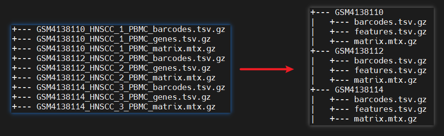
0、导入数据方式
(1)cellranger比对结果
对每个测序样本数据经cellranger上游比对,产生3个文件,分别是:
- barcodes.tsv.gz – 细胞标签
- features.tsv.gz – 基因名
- matrix.mtx.gz – 表达数据
|
|
(2)直接提供表达矩阵
|
|
(3)h5格式文件
|
|
(4)h5ad格式
- 需要安装,使用
SeuratDisk包的两个函数; - 先将后
h5ad格式转换为h5seurat格式,再使用LoadH5Seurat()函数读取Seurat对象。
|
|
- 将Seurat对象转为h5ad格式
|
|
(5)10X PBMC demo
|
|
1、批量创建Seurat对象
(1)规范化10X文件样本名
每个样本一个文件夹,分别包含三个文件:barcodes.tsv.gz, features.tsv.gz, matrix.mtx.gz
|
|
(2)合并多样本
|
|
(3)过滤细胞/基因
|
|
2、标归高降维
(1)标归高
标准化–归一化–鉴定高变基因
|
|
(2)降维聚类分群
|
|
3、Seurat结构
|
|
|
|
4、Seurat可视化
|
|
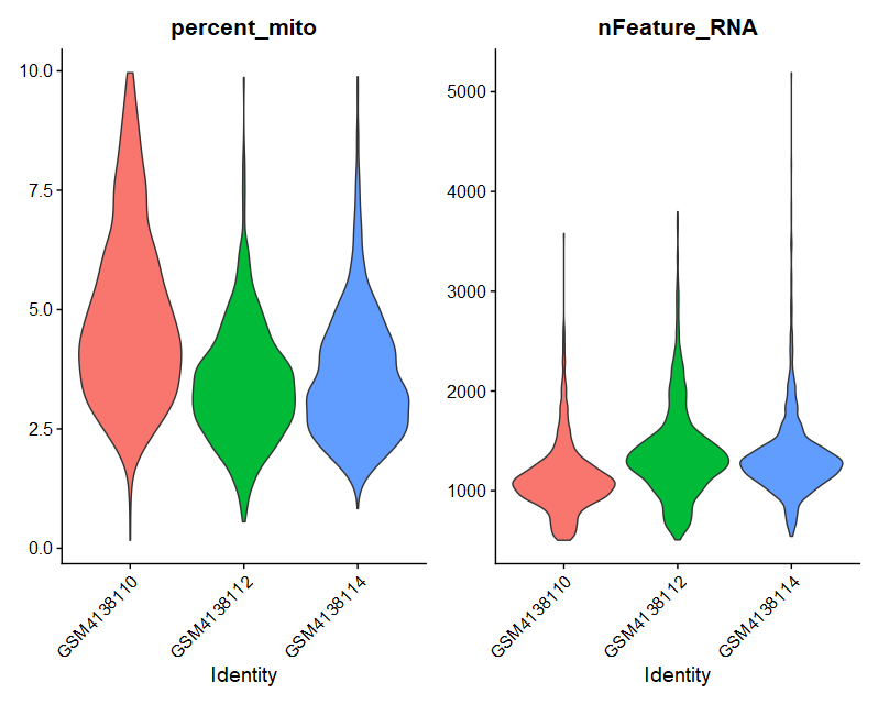
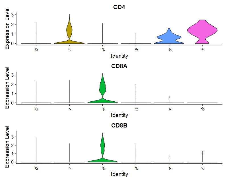
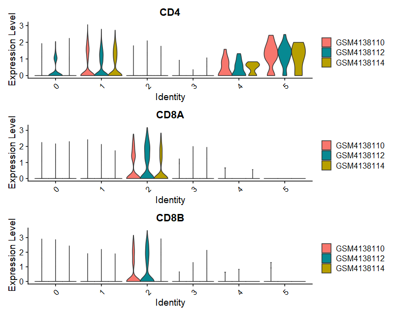
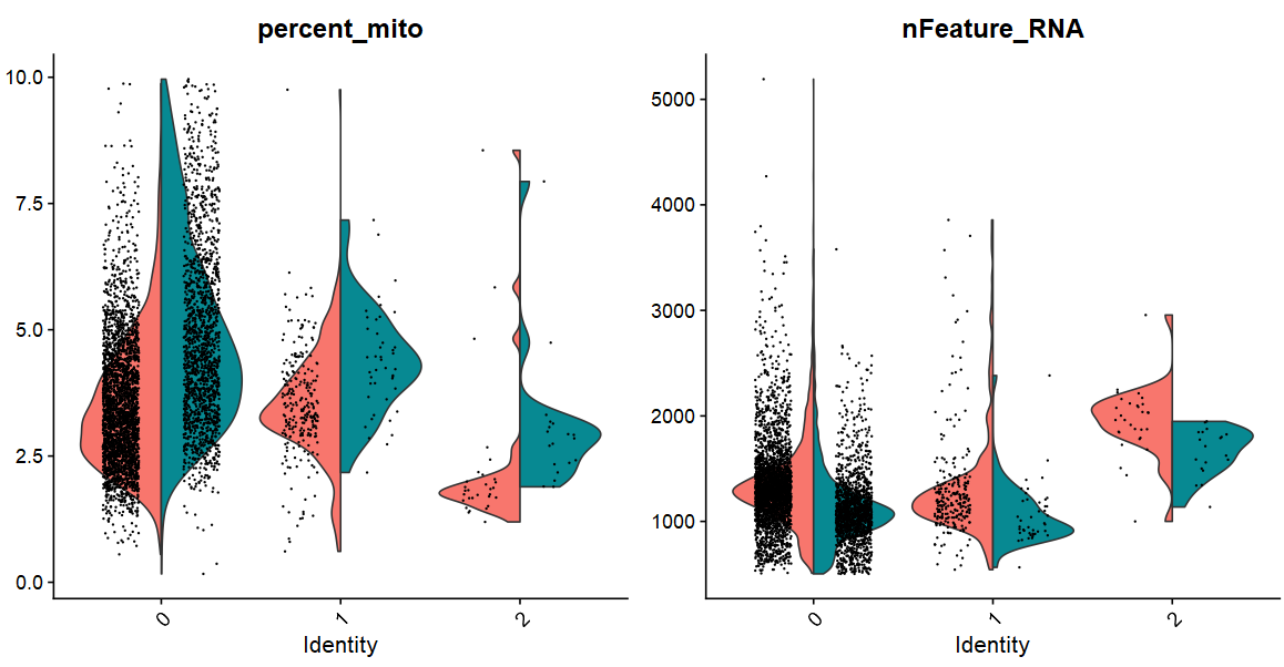
(1)VlnPlot
|
|
|
|
|
|
|
|
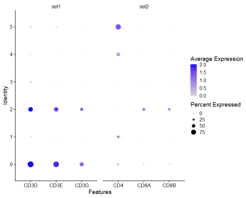
(2)DotPlot
|
|
|
|
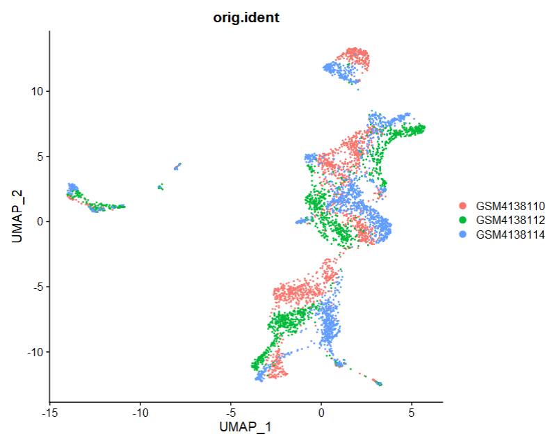
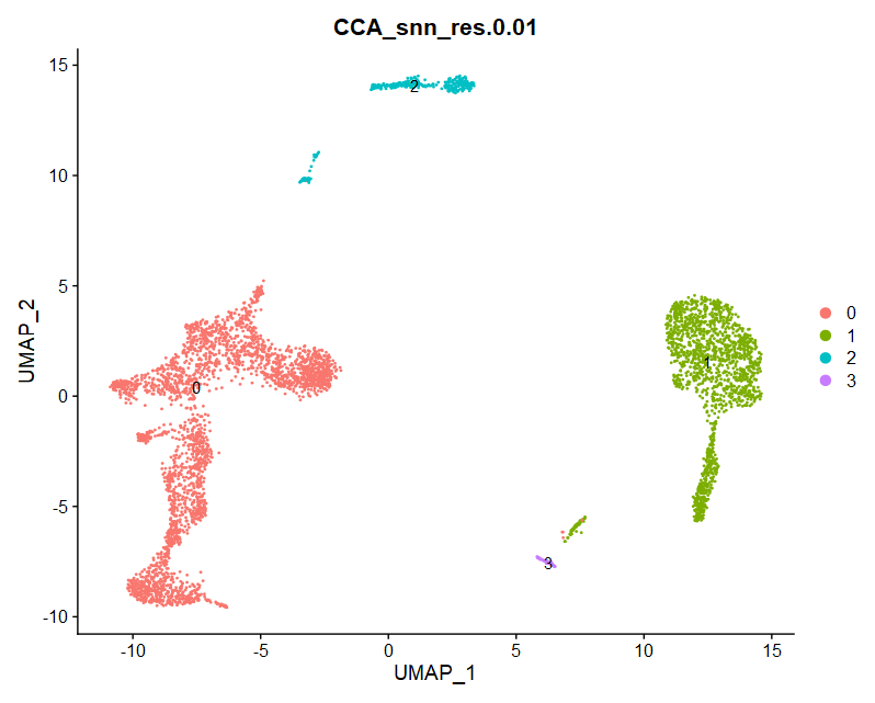
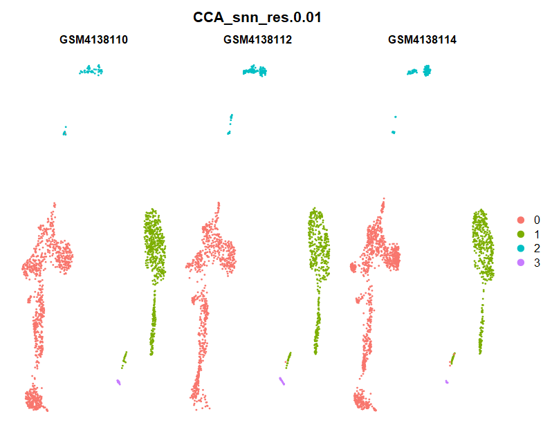
(3)Dimplot
|
|
|
|
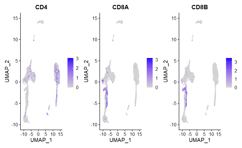
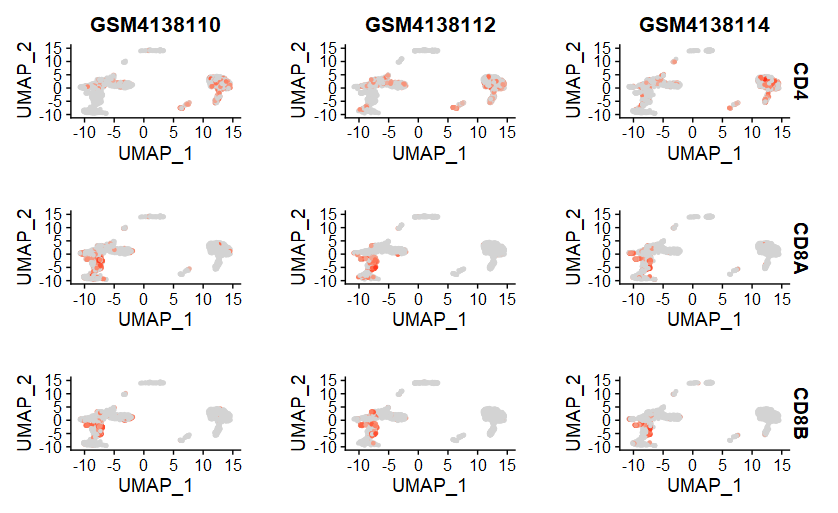
(4)FeaturePlot
|
|
|
|
5、注释细胞类型
- marker基因:Dotplot
- 假设根据CCA_snn_res.0.05分群结果,将6个cluster注释为4中细胞类型
|
|
6、差异分析
|
|
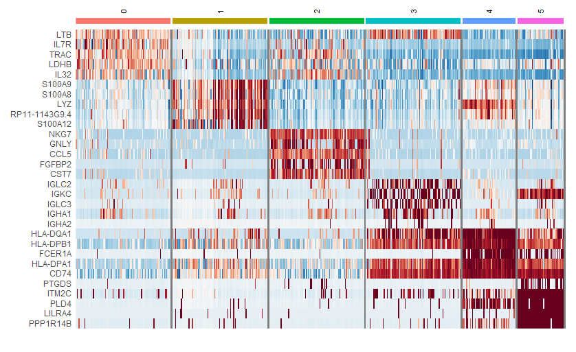
(1)FindAllMarkers
|
|
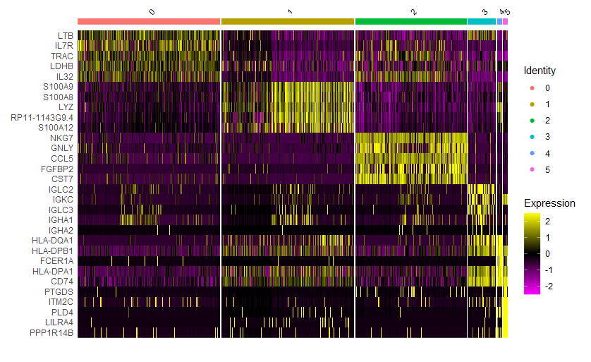
|
|
(2)FindMarkers
|
|
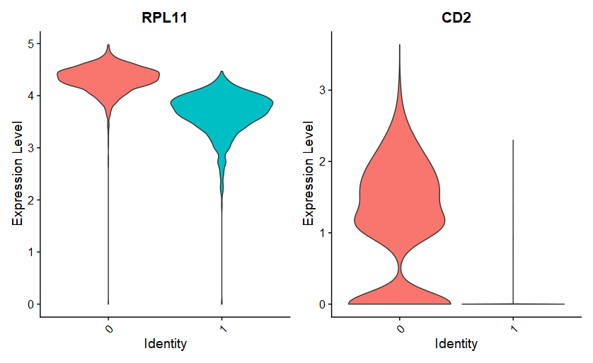
|
|
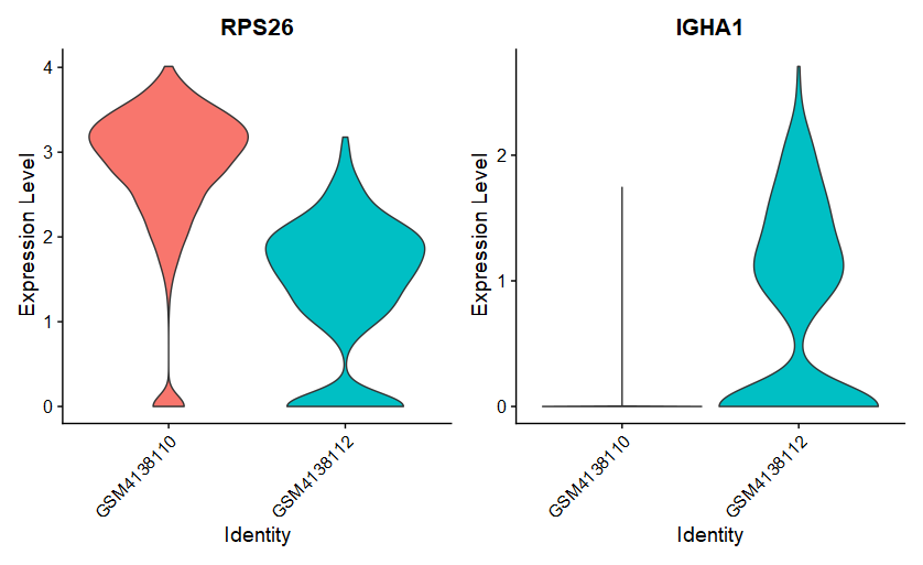
(3)FindConservedMarkers
|
|
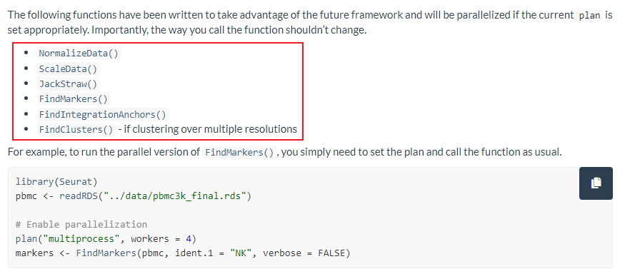
7、多线程
|
|
8、基因集打分
|
|