1、算法简介

1.1 关系拆解

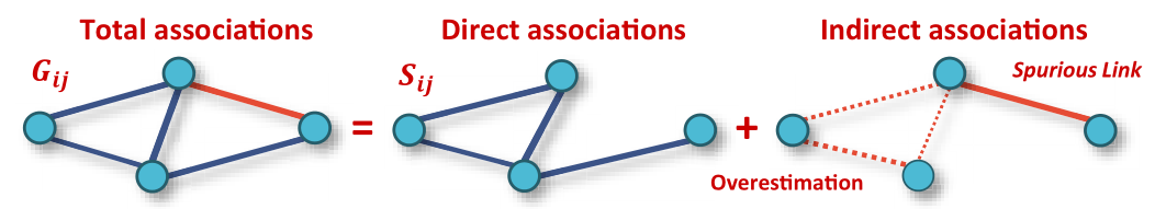
通过计算方法( 例如相关性Pearson correlation, 互信息mutual information等)构建的相互关系网络中，节点两两之间的关系通常包括直接关系与间接关系两部分，即如下图所示Total = Direct + Indirect

PNAS的一篇文章提供了一种从计算网络中鉴定节点之间direct association的新方法–iDIRECT(Inference of Direct and Indirect Relationships with Effective Copula-based Transitivity)

Disentangling direct from indirect relationships in association networks

DOI: 10.1073/pnas.2109995119

PNAS 2022 Jan 11

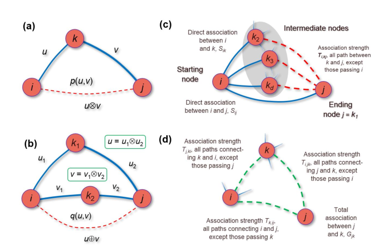
对于Sequential paths(如下图A)，即两个节点之间存在1至多个中间节点连接二者。可通过简单的关系乘法计算这两个节点在这条path的indirect关系。

$$ u \otimes v = uv $$

对于parallel paths中(如下图B)，即两个节点之间存在多条path。此时并没有简单的相加，而是采用Archimedean copulas计算 combined probability。从而保证u⊕v ∈ [0,1] for all u,v ∈ [0,1]。其中u、v表示每条path的indirect association

$$ u\oplus v = \frac{u+v-2uv}{1-uv} $$

对于存在direct与indirect association的节点对。其中G表示observation association；S表示direct association

$$ G_{ij} = S_{ij}\oplus S_{ik_2}G_{k_2j} \oplus S_{ik_3}G_{k_3j} \oplus … \oplus S_{ik_d}G_{k_dj} $$

文章对上式做了进一步的改进：在计算节点i的邻居k(假如为k2)与节点j的关系时，排除self-looping path(k-i-j)后再进行计算k2与j的total association。

$$ G_{ij} = S_{ij}\oplus S_{ik_2}T_{i,k_2j} \oplus S_{ik_3}T_{i,k_3j} \oplus … \oplus S_{ik_d}T_{i,k_dj} $$

1.2 算法对比

文中提到之前已经有人提出相关方法，例如network deconvolution (ND)、global silencing (GS)等

作者认为以前的方法中存在3点不足

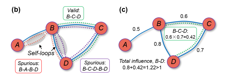
（1）interaction strength overﬂow：对于parallel path采用简单的相加，可能会存在 over-estimation。
- 本文采用了Archimedean copulas方式计算多条path之和（如上图b所示）
（2）self-looping：对于indirect association，考虑了包含自身的冗余路径。
- 本文提出在计算indirect path时，一种计算transitivity matrix的新思路，用以去冗余。（如上图c所示）
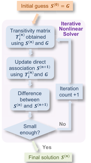
（3） ill-conditioning：对于这一点，暂时没有太理解。作者认为ND、GS等方法求解 direct association时借助转置矩阵G-1。但由于关系矩阵一般近奇异，转置操作具有高度不确定性。而本文使用了称为nonlinear solver方法，进行推算迭代、直至稳定。

Specifically, ill-conditioning means that the association matrix is close to singular and is highly unreliable to invert.

2、Python脚本

作者已将代码封装为Python脚本，可直接使用。

https://github.com/nxiao6gt/iDIRECT
为了适应不同python版本，作者提供了对应python版本的脚本文件

 1
 2
 3
 4
 5
 6
 7
 8
 9
10
11
12
13
14
15
16
17
18
19
20
21
22
23
24
25
26
27
28
29
30
31
32
33
34
35
36
37
38
39
40
41
42
43
44
45
46
47
48
49
50
51
52
53
54
55
56
57
58
59
60
61
62
63
64
65
66
67
68
69


git clone https://github.com/nxiao6gt/iDIRECT.git
# iDIRECT/
# ├── demo.py
# ├── file_handler.pyc
# ├── idirect.pyc          ##主要分析脚本，默认为3.8版本的
# ├── LICENSE
# ├── net_handler.pyc
# ├── net_simulator.pyc
# ├── __pycache__
# ├── README.md
# ├── result
# ├── script
# └── versions

tree iDIRECT/versions/
# iDIRECT/versions/
# ├── 3.5
# │   ├── file_handler.pyc
# │   ├── idirect.pyc
# │   ├── net_handler.pyc
# │   └── net_simulator.pyc
# ├── 3.8
# │   ├── file_handler.pyc
# │   ├── idirect.pyc
# │   ├── net_handler.pyc
# │   └── net_simulator.pyc
# └── 3.9
    # ├── file_handler.pyc
    # ├── idirect.pyc
    # ├── net_handler.pyc
    # └── net_simulator.pyc
    
##(1) 选择相应版本的python脚本 
ls iDIRECT/versions/3.8/*pyc | while read id ; do cp ${id} iDIRECT/; done
cd iDIRECT
#进入Python环境
import idirect as idir
import file_handler as fh
import net_handler as nh
from time import time
t0 = time()

##(2) 准备observable total association matrix G
# cat result/demo.txt 
# N1      N2      0.7
# N2      N3      0.7
# N1      N3      0.5
# 如上是3个节点、3条边的total association matrix
# 读取矩阵，以字典的形式存放
G,n = fh.read_file_weighted_edges("result/demo.txt", t0) 
G
# {'N1': {'N2': 0.7, 'N3': 0.5},
#  'N2': {'N1': 0.7, 'N3': 0.7},
#  'N3': {'N2': 0.7, 'N1': 0.5}}

##(3) 计算direct association network
S,err = idir.direct_association(G, t0=t0)
# {'N1': {'N2': 0.6963451220087372, 'N3': 0.055394034573922085},
#  'N2': {'N1': 0.6963451220087372, 'N3': 0.6963451220087373},
#  'N3': {'N2': 0.6963451220087373, 'N1': 0.055394034573922085}}

##(4) 保存结果 direct association matrix S
S2 = nh.merge(G, S)
St = fh.save_sorted_turple(S2, in_file="result/demo.txt")
fh.save_file_weighted_edges(St, "result/demo_res.txt")
# cat result/demo_res.txt 
# N1      N2      0.696345122
# N2      N3      0.696345122
# N1      N3      0.055394035

3、应用示例

在文章Result中除了第一部分简单介绍了iDIRECT的算法原理，后续部分都是通过在不同类型/背景网络中的应用（同时对比其它算法）说明本方法的优势。

简单介绍一下在优化基因调控网络关系中的示例：

3.1 DREAM5

DREAM5有一项重构基因网络挑战项目，其中有一个模拟的基因表达数据(GeneNet-Weaver (GNW) version 3.0)，同时给出了gold-standard 基因调控关系（0/1）。参赛者采用不同的计算方法试图重构网络，然后DREAM5基于gold-standard对预测结果进行评价。

评价方式是从0到1遍历不同cut-off得到的true-positive rate/false-negative rate得到的AUPR与AUROC。
然后进行随机1,000 random simulations，得到的AUPR与AUROC分布，作为背景，从而计算上述方法得到的AUPR与AUROC的P值

原文描述为：

Those links were then scored based on the true network using the Challenge organizer’s script (details in Mate- rials and Methods), which was just -log(p) of the empirical P-values of the predicted AUPR from 1,000 random simulations.

3.2 iDIRECT优化

文章对于参赛者已提交的、基于不同算法得到network使用iDIRECT，以期望从中鉴定出direct association；
同时对比ND与GS两种方法的结果；
在结果评价上，同时考虑了AUPR与AUROC两个指标

$$ \Theta_{PR} = -log_{10}P_{PR} $$

$$ \Theta_{ROC} = -log_{10}P_{ROC} $$

$$ \Theta_{total} = (\Theta_{PR} + \Theta_{ROC})/2 $$

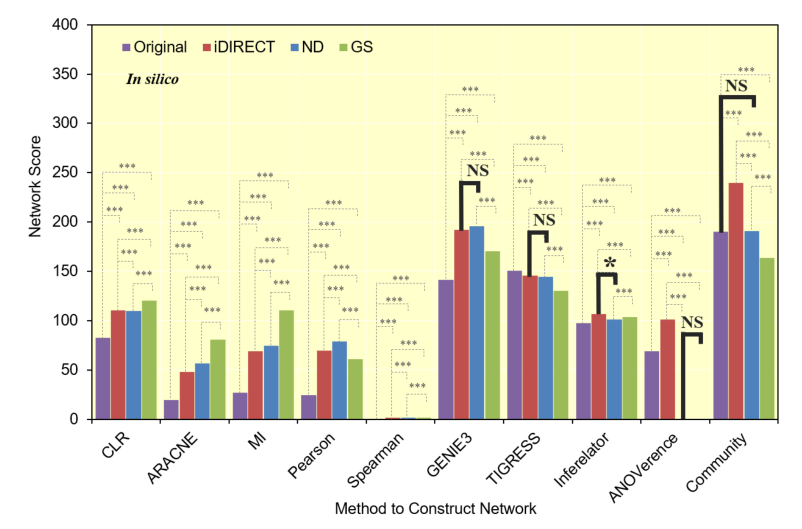
AUPR represents the average precision when recall (true-positive rate) varies from zero to one;

AUROC represents the average true positive rate when the false-negative rate varies from zero to one.

1、算法简介#

1.1 关系拆解#

1.2 算法对比#

2、Python脚本#

3、应用示例#

3.1 DREAM5#

3.2 iDIRECT优化#