1
2
3
4
5
6
7
8
9
10
11
12
13
14
15
16
17
18
19
20
|
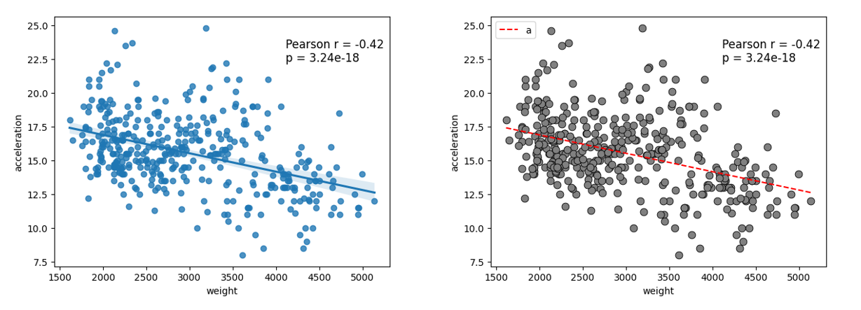
# 数据准备
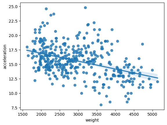
mpg = sns.load_dataset("mpg").dropna(subset=["weight", "acceleration"])
x = mpg["weight"]
y = mpg["acceleration"]
# 绘制散点
sns.scatterplot(x=x, y=y, color="gray", edgecolor="black", s=60)
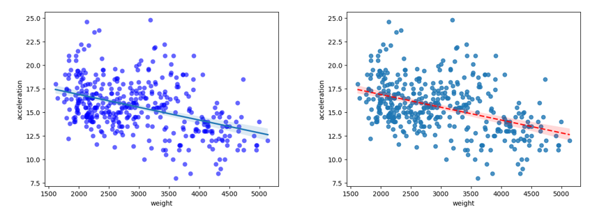
# 添加回归线(用 numpy.polyfit)
slope, intercept = np.polyfit(x, y, deg=1)
x_vals = np.linspace(x.min(), x.max(), 100)
y_vals = slope * x_vals + intercept
plt.plot(x_vals, y_vals, color="red", linestyle="--", label="Linear fit")
# 添加相关性注释
r, p = pearsonr(x, y)
plt.text(x.max()*0.8, y.max()*0.9, f"Pearson r = {r:.2f}\np = {p:.2e}", fontsize=12)
plt.legend()
plt.show()
|